Quick survey of some other important concepts in geo-data-science

The field of data science for Earth sciences is vast, and the available software tools are always growing and changing. If you end up using these tools in your work, you can (and should) expect to keep learning and refining your skills and toolbox. This also means that no single course can cover everything (specially not a 6 week course).

In this notebook we will get a high level overview of a few more concepts (software packages), which may be helpful as starting points for further exploration.

Maps

This is a derivative of the longer notebook available here.

Making maps is a fundamental part of geoscience research. Maps differ from regular figures in the following principle ways:

• Maps require a projection of geographic coordinates on the 3D Earth to the 2D space of your figure.

• Maps often include extra decorations besides just our data (e.g. continents, country borders, etc.)

Mapping is a notoriously hard and complicated problem, mostly due to the complexities of projection.

In this lecture, we will learn about Cartopy, one of the most common packages for making maps within python.

Projections: Most of our media for visualization are flat

Our two most common media are flat:

• Paper

• Screen

[Map] Projections: Taking us from spherical to flat

A map projection (or more commonly refered to as just “projection”) is:

a systematic transformation of the latitudes and longitudes of locations from the surface of a sphere or an ellipsoid into locations on a plane. [Wikipedia: Map projection].

The major problem with map projections

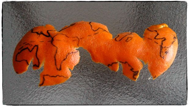
• The surface of a sphere is topologically different to a 2D surface, therefore we have to cut the sphere somewhere

• A sphere’s surface cannot be represented on a plane without distortion.

There are many different ways to make a projection, and we will not attempt to explain all of the choices and tradeoffs here. Instead, you can read Phil’s original tutorial for a great overview of this topic. Instead, we will dive into the more practical sides of Caropy usage.

Introducing Cartopy

https://scitools.org.uk/cartopy/docs/latest/

Cartopy makes use of the powerful PROJ.4, numpy and shapely libraries and includes a programatic interface built on top of Matplotlib for the creation of publication quality maps.

Key features of cartopy are its object oriented projection definitions, and its ability to transform points, lines, vectors, polygons and images between those projections.

import cartopy.crs as ccrs
import cartopy

ccrs.PlateCarree()

<cartopy.crs.PlateCarree object at 0x79e910270cb0>

# Can use with matplotlib 
%matplotlib inline
import matplotlib.pyplot as plt

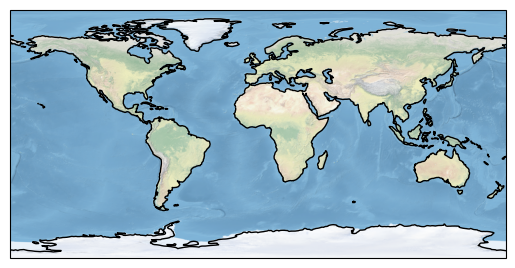
ax = plt.axes(projection=ccrs.PlateCarree())
ax.coastlines()
ax.stock_img()

<matplotlib.image.AxesImage at 0x79e86ffa75c0>

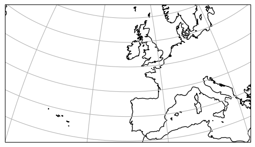
# Can make regional maps 
central_lon, central_lat = -10, 45
extent = [-40, 20, 30, 60]
ax = plt.axes(projection=ccrs.Orthographic(central_lon, central_lat))
ax.set_extent(extent)
ax.gridlines()
ax.coastlines(resolution='50m')

<cartopy.mpl.feature_artist.FeatureArtist at 0x79e86ff60800>

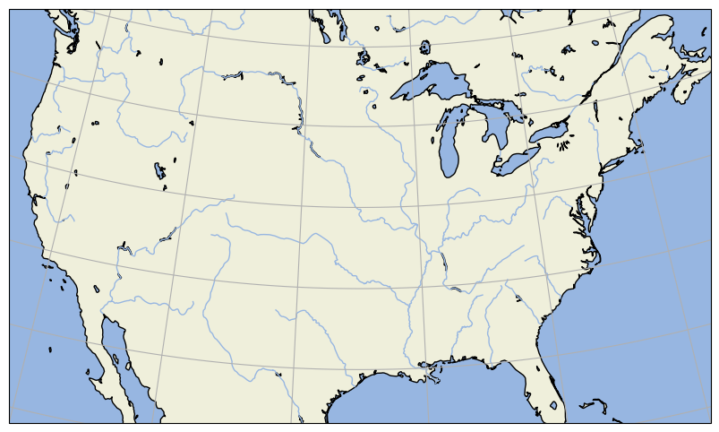
# Can add some default features 
import cartopy.feature as cfeature
import numpy as np

central_lat = 37.5
central_lon = -96
extent = [-120, -70, 24, 50.5]
central_lon = np.mean(extent[:2])
central_lat = np.mean(extent[2:])

plt.figure(figsize=(12, 6))
ax = plt.axes(projection=ccrs.AlbersEqualArea(central_lon, central_lat))
ax.set_extent(extent)

ax.add_feature(cartopy.feature.OCEAN)
ax.add_feature(cartopy.feature.LAND, edgecolor='black')
ax.add_feature(cartopy.feature.LAKES, edgecolor='black')
ax.add_feature(cartopy.feature.RIVERS)
ax.gridlines()

<cartopy.mpl.gridliner.Gridliner at 0x79e867e354c0>

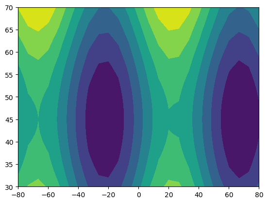
import numpy as np
lon = np.linspace(-80, 80, 25)
lat = np.linspace(30, 70, 25)
lon2d, lat2d = np.meshgrid(lon, lat)
data = np.cos(np.deg2rad(lat2d) * 4) + np.sin(np.deg2rad(lon2d) * 4)
plt.contourf(lon2d, lat2d, data)

<matplotlib.contour.QuadContourSet at 0x79e867e67890>

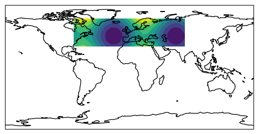
ax = plt.axes(projection=ccrs.PlateCarree())
ax.set_global()
ax.coastlines()
ax.contourf(lon, lat, data)

<cartopy.mpl.contour.GeoContourSet at 0x79e8664df920>

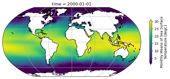
# Integration with xarray

import xarray as xr
url = 'http://www.esrl.noaa.gov/psd/thredds/dodsC/Datasets/noaa.ersst.v5/sst.mnmean.nc'
ds = xr.open_dataset(url, drop_variables=['time_bnds'])
sst = ds.sst.sel(time='2000-01-01', method='nearest')
fig = plt.figure(figsize=(9,6))
ax = plt.axes(projection=ccrs.Robinson())
ax.coastlines()
ax.gridlines()
sst.plot(ax=ax, transform=ccrs.PlateCarree(),
         vmin=2, vmax=30, cbar_kwargs={'shrink': 0.4})

<cartopy.mpl.geocollection.GeoQuadMesh at 0x79e8434cf1d0>

Earth Science Model (ESM) Output

ESMs are computer models, which approximately model the earth system. These types of models are used in a variety of contexts in the Earth Science: From idealized experiments to understand meachanisms in the climate systems, to reanalyses and state estimates to synthesize past and current observations, to fully coupled representations of the earth system enabling forecasts of climate conditions under future scenarios.

What is a General Circulation Model?

A GCM is a computer model that simulates the circulation of a fluid (e.g., the ocean or atmosphere), and is thus one (but important) component of an ESM. It is based on a set of partial differential equations, which describe the motion of a fluid in 3D space, and integrates these forward in time. Most fundamentally, these models use a discrete representation of the Navier-Stokes Equations but can include more equations to represent e.g., the thermodynamics, chemistry or biology of the coupled earth system. Depending on the goal these equations are forced with predetermined boundary conditions (e.g. an ocean only simulation is forced by observed atmospheric conditions) or the components of the earth system are coupled together and allowed to influence each other. A ‘climate model’ is often the latter case which is forced by e.g. different scenarios of greenhouse gas emissions. This enables predictions of how the coupled system will evolve in the future.

The globe divided into boxes

Since there is no analytical solution to the full Navier-Stokes equation, modern GCMs solve them using numerical methods. They use a discretized version of the equations, which approximates them within a finite volume, or grid-cell. Each GCM splits the ocean or atmosphere into many cells, both in the horizontal and vertical.

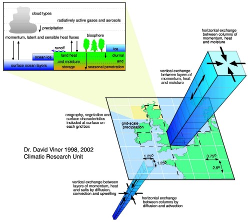
Source: www.ipcc-data.org

It is numerically favorable to shift (or ‘stagger’) the grid points where the model calculates the velocity with regard to the grid point where tracer values (temperature, salinity, or others) are calculated. There are several different ways to shift these points, commonly referred to as Arakawa grids.

Source: xgcm.readthedocs.io

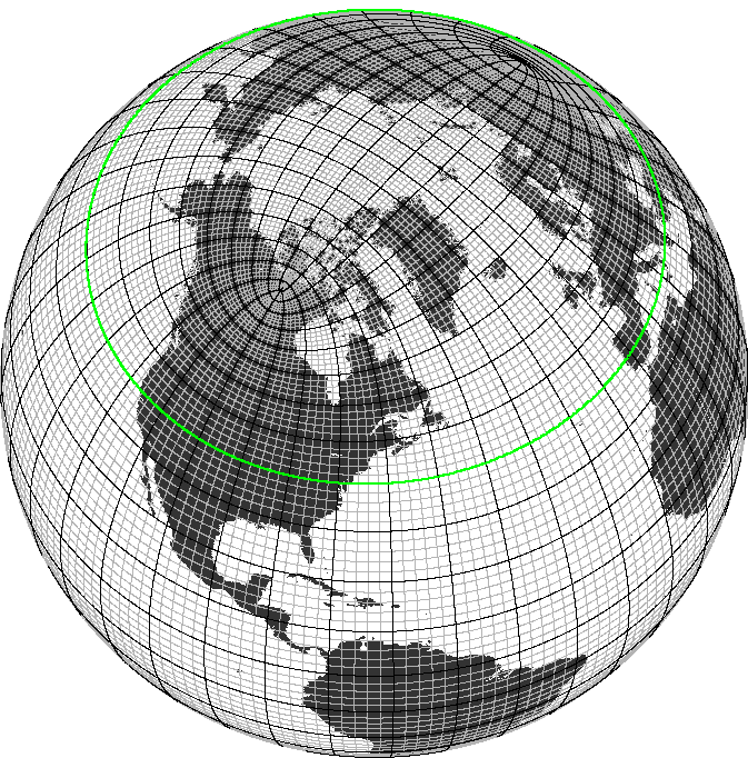
Most GCMs use a curvilinear grid to avoid infinitely small grid cells at the North Pole. Some examples of curvilinear grids are a tripolar grid (the Arctic region is defined by two poles, placed over landmasses)

Source: GEOMAR

or a cubed-sphere grid or a lat-lon cap (different versions of connected patches of curvilinear grids).

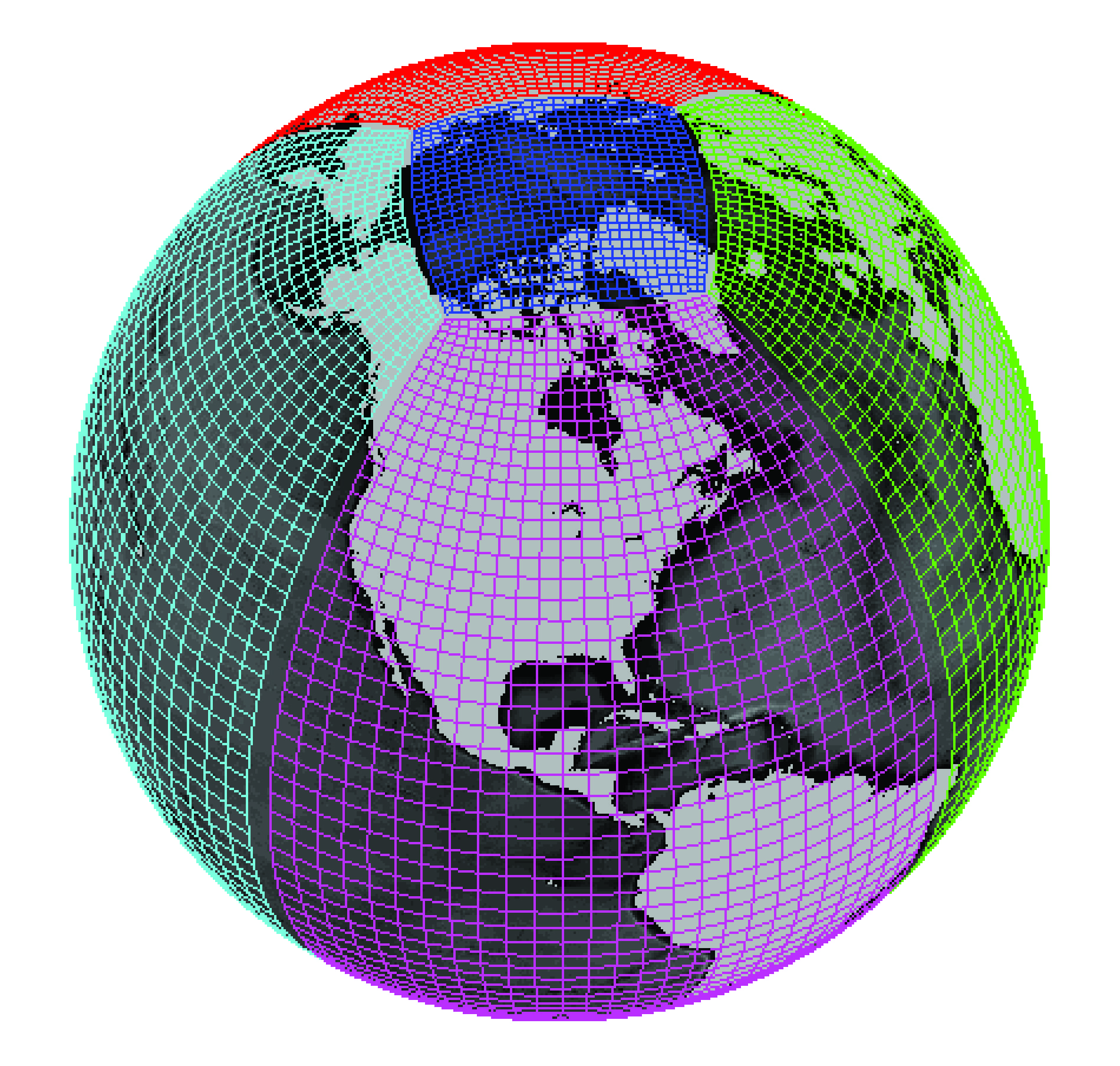
Credit: Gael Forget. More information about the simulation and grid available at https://doi.org/10.5194/gmd-8-3071-2015.

In most ocean models, due to these ‘warped’ coordinate systems, the boxes described are not perfectly rectangular cuboids. To accurately represent the volume of the cell, we require so-called grid metrics - the distances, cell areas, and volume to calculate operators like e.g., divergence.

If you want to compare models with different grids it can sometimes be necessary to regrid your output. However, some calculations should be performed on the native model grid for maximum accuracy. We will discuss these different cases below.

Grid resolution

Discretizing the equations has consequences:

• In order to get a realistic representation of the global circulation, the size of grid cells needs to be chosen so that all relevant processes are resolved. In reality, this usually requires too much computing power for global models and so processes that are too small to be explicitly resolved, like mesoscale eddies or vertical mixing, need to be carefully parameterized since they influence the large scale circulation. The following video illustrates the representation of mesoscale eddies in global models of different grid resolution. It shows the surface nutrient fields of three coupled climate models (produced by NOAA/GFDL) around the Antarctic Peninsula with increasing ocean resolution from left to right.

Nominal model resolution from left to right: 1 degree (CM2.1deg), 0.25 degree (CM2.5) and 0.1 degree (CM2.6). The left ocean model employs a parametrization for both the advective and diffusive effects of mesoscale eddies, while the middle and right model do not.

CMIP - Climate Model Intercomparison Project

Climate modeling has been a cornerstone of understanding our climate and the consequences of continued emissions of greenhouse gases for decades. Much of the recent efforts in the community have been focus on model intercomparison projects (MIPs), which invite submissions of many different modeling groups around the world to run their models (which are all set up slightly different) under centralized forcing scenarios. These results can then be analyzed and the spread between different models can give an idea about the certainty of these predictions. The recent Coupled Model Intercomparison Project Phase 6 (CMIP6) represents an international effort to represent the state-of-the-art knowledge about how the climate system might evolve in the future and informs much of the [Intergovernmental Panel on Climate Change Report](Intergovernmental Panel on Climate Change Report.

In this lecture we will learn how to quickly search and analyze CMIP6 data with Pangeo tools in the cloud, a process that using the ‘download and analyze’ workflow often becomes prohibitively slow and inefficient due to the sheer scale of the data.

The basis for this workflow are the analysis-ready-cloud-optimized repositories of CMIP6 data, which are currently maintained by the pangeo community and publicly available on both Google Cloud Storage and Amazon S3 as a collection of zarr stores.

The cloud native approach enables scientific results to be fully reproducible, encouraging to build onto and collaborate on scientific results.

Here we use a Python library called xmip.

from xmip.preprocessing import combined_preprocessing
from xmip.utils import google_cmip_col
from xmip.postprocessing import match_metrics
import matplotlib.pyplot as plt

The first thing we have to do is to get an overview of all the data available. In this case we are using intake-esm to load a collection of zarr stores on Google Cloud Storage, but there are other options to access the data too.

Lets create a collection object and look at it

col = google_cmip_col()
col

Future exception was never retrieved
future: <Future finished exception=ClientConnectionError('Connection lost: [SSL: APPLICATION_DATA_AFTER_CLOSE_NOTIFY] application data after close notify (_ssl.c:2706)')>
Traceback (most recent call last):
  File "/srv/conda/envs/notebook/lib/python3.12/asyncio/sslproto.py", line 651, in _do_shutdown
    self._sslobj.unwrap()
  File "/srv/conda/envs/notebook/lib/python3.12/ssl.py", line 920, in unwrap
    return self._sslobj.shutdown()
           ^^^^^^^^^^^^^^^^^^^^^^^
ssl.SSLError: [SSL: APPLICATION_DATA_AFTER_CLOSE_NOTIFY] application data after close notify (_ssl.c:2706)

The above exception was the direct cause of the following exception:

aiohttp.client_exceptions.ClientConnectionError: Connection lost: [SSL: APPLICATION_DATA_AFTER_CLOSE_NOTIFY] application data after close notify (_ssl.c:2706)

pangeo-cmip6 catalog with 7674 dataset(s) from 514818 asset(s):

	unique
activity_id	18
institution_id	36
source_id	88
experiment_id	170
member_id	657
table_id	37
variable_id	700
grid_label	10
zstore	514818
dcpp_init_year	60
version	736
derived_variable_id	0

This object describes all the available data (over 500k single zarr stores!). The rows describe different ‘facets’ that can be used to search and query subsets of the data. For detailed info on each of the facets please refer to this document.

So obviously we never want to work with all the data. Lets check out how to get a subset.

First we need to understand a bit better what all these facets mean and how to see which ones are in the full collection. Lets start with the experiment_id: This is the prescribed forcing for a particular MIP that is exactly the same across all different models. We can look at the values of the collection as a pandas dataframe to convieniently list all values.

col.df['experiment_id'].unique()

array(['highresSST-present', 'piControl', 'control-1950', 'hist-1950',
       'historical', 'amip', 'abrupt-4xCO2', 'abrupt-2xCO2',
       'abrupt-0p5xCO2', '1pctCO2', 'ssp585', 'esm-piControl', 'esm-hist',
       'hist-piAer', 'histSST-1950HC', 'ssp245', 'hist-1950HC', 'histSST',
       'piClim-2xVOC', 'piClim-2xNOx', 'piClim-2xdust', 'piClim-2xss',
       'piClim-histall', 'hist-piNTCF', 'histSST-piNTCF',
       'aqua-control-lwoff', 'piClim-lu', 'histSST-piO3', 'piClim-CH4',
       'piClim-NTCF', 'piClim-NOx', 'piClim-O3', 'piClim-HC',
       'faf-heat-NA0pct', 'ssp370SST-lowCH4', 'piClim-VOC',
       'ssp370-lowNTCF', 'piClim-control', 'piClim-aer', 'hist-aer',
       'faf-heat', 'faf-heat-NA50pct', 'ssp370SST-lowNTCF',
       'ssp370SST-ssp126Lu', 'ssp370SST', 'ssp370pdSST', 'histSST-piAer',
       'piClim-ghg', 'piClim-anthro', 'faf-all', 'hist-nat', 'hist-GHG',
       'ssp119', 'piClim-histnat', 'piClim-4xCO2', 'ssp370',
       'piClim-histghg', 'highresSST-future', 'esm-ssp585-ssp126Lu',
       'ssp126-ssp370Lu', 'ssp370-ssp126Lu', 'land-noLu', 'histSST-piCH4',
       'ssp126', 'esm-pi-CO2pulse', 'amip-hist', 'piClim-histaer',
       'amip-4xCO2', 'faf-water', 'faf-passiveheat', '1pctCO2-rad',
       'faf-stress', '1pctCO2-bgc', 'aqua-control', 'amip-future4K',
       'amip-p4K', 'aqua-p4K', 'amip-lwoff', 'amip-m4K', 'aqua-4xCO2',
       'amip-p4K-lwoff', 'hist-noLu', '1pctCO2-cdr',
       'land-hist-altStartYear', 'land-hist', 'omip1', 'esm-pi-cdr-pulse',
       'esm-ssp585', 'abrupt-solp4p', 'piControl-spinup', 'hist-stratO3',
       'abrupt-solm4p', 'midHolocene', 'lig127k', 'aqua-p4K-lwoff',
       'esm-piControl-spinup', 'ssp245-GHG', 'ssp245-nat',
       'dcppC-amv-neg', 'dcppC-amv-ExTrop-neg', 'dcppC-atl-control',
       'dcppC-amv-pos', 'dcppC-ipv-NexTrop-neg', 'dcppC-ipv-NexTrop-pos',
       'dcppC-atl-pacemaker', 'dcppC-amv-ExTrop-pos',
       'dcppC-amv-Trop-neg', 'dcppC-pac-control', 'dcppC-ipv-pos',
       'dcppC-pac-pacemaker', 'dcppC-ipv-neg', 'dcppC-amv-Trop-pos',
       'piClim-BC', 'piClim-2xfire', 'piClim-SO2', 'piClim-OC',
       'piClim-N2O', 'piClim-2xDMS', 'ssp460', 'ssp434', 'ssp534-over',
       'deforest-globe', 'historical-cmip5', 'hist-bgc',
       'piControl-cmip5', 'rcp26-cmip5', 'rcp45-cmip5', 'rcp85-cmip5',
       'pdSST-piArcSIC', 'pdSST-piAntSIC', 'piSST-piSIC', 'piSST-pdSIC',
       'ssp245-stratO3', 'hist-sol', 'hist-CO2', 'hist-volc',
       'hist-totalO3', 'hist-nat-cmip5', 'hist-aer-cmip5',
       'hist-GHG-cmip5', 'pdSST-futAntSIC', 'futSST-pdSIC', 'pdSST-pdSIC',
       'ssp245-aer', 'pdSST-futArcSIC', 'dcppA-hindcast', 'dcppA-assim',
       'dcppC-hindcast-noPinatubo', 'dcppC-hindcast-noElChichon',
       'dcppC-hindcast-noAgung', 'ssp245-cov-modgreen',
       'ssp245-cov-fossil', 'ssp245-cov-strgreen', 'ssp245-covid', 'lgm',
       'ssp585-bgc', '1pctCO2to4x-withism', '1pctCO2-4xext',
       'hist-resIPO', 'past1000', 'pa-futArcSIC', 'pa-pdSIC',
       'historical-ext', 'pdSST-futArcSICSIT', 'pdSST-futOkhotskSIC',
       'pdSST-futBKSeasSIC', 'pa-piArcSIC', 'pa-piAntSIC', 'pa-futAntSIC',
       'pdSST-pdSICSIT'], dtype=object)

The experiments you are probably most interested in are the following:

• piControl: In most cases this is the ‘spin up’ phase of the model, where it is run with a constant forcing (representing pre-industrial greenhouse gas concentrations)

• historical: This experiment is run with the observed forcing in the past.

• ssp***: A set of “Shared Socioeconomic Pathways” which represent different combined scenarios of future greenhouse gas emissions and other socio-economic indicators (Explainer). These are a fairly complex topic, but to simplify this for our purposes here we can treat ssp585 as the ‘worst-case’ and ssp245 as ‘middle-of-the-road’.

You can explore the available models (source_id) in the same way as above:

col.df['source_id'].unique()

array(['CMCC-CM2-HR4', 'EC-Earth3P-HR', 'HadGEM3-GC31-MM',
       'HadGEM3-GC31-HM', 'HadGEM3-GC31-LM', 'EC-Earth3P', 'ECMWF-IFS-HR',
       'ECMWF-IFS-LR', 'HadGEM3-GC31-LL', 'CMCC-CM2-VHR4', 'GFDL-CM4',
       'GFDL-AM4', 'IPSL-CM6A-LR', 'E3SM-1-0', 'CNRM-CM6-1', 'GFDL-ESM4',
       'GFDL-ESM2M', 'GFDL-CM4C192', 'GFDL-OM4p5B', 'GISS-E2-1-G',
       'GISS-E2-1-H', 'CNRM-ESM2-1', 'BCC-CSM2-MR', 'BCC-ESM1', 'MIROC6',
       'AWI-CM-1-1-MR', 'EC-Earth3-LR', 'IPSL-CM6A-ATM-HR', 'CESM2',
       'CESM2-WACCM', 'CNRM-CM6-1-HR', 'MRI-ESM2-0', 'SAM0-UNICON',
       'GISS-E2-1-G-CC', 'UKESM1-0-LL', 'EC-Earth3', 'EC-Earth3-Veg',
       'FGOALS-f3-L', 'CanESM5', 'CanESM5-CanOE', 'INM-CM4-8',
       'INM-CM5-0', 'NESM3', 'MPI-ESM-1-2-HAM', 'CAMS-CSM1-0',
       'MPI-ESM1-2-LR', 'MPI-ESM1-2-HR', 'MRI-AGCM3-2-H', 'MRI-AGCM3-2-S',
       'MCM-UA-1-0', 'INM-CM5-H', 'KACE-1-0-G', 'NorESM2-LM',
       'FGOALS-f3-H', 'FGOALS-g3', 'MIROC-ES2L', 'FIO-ESM-2-0', 'NorCPM1',
       'NorESM1-F', 'MPI-ESM1-2-XR', 'CESM1-1-CAM5-CMIP5', 'E3SM-1-1',
       'KIOST-ESM', 'ACCESS-CM2', 'NorESM2-MM', 'ACCESS-ESM1-5',
       'IITM-ESM', 'GISS-E2-2-G', 'CESM2-FV2', 'GISS-E2-2-H',
       'CESM2-WACCM-FV2', 'CIESM', 'E3SM-1-1-ECA', 'TaiESM1',
       'AWI-ESM-1-1-LR', 'EC-Earth3-Veg-LR', 'CMCC-ESM2', 'CMCC-CM2-SR5',
       'EC-Earth3-AerChem', 'IPSL-CM6A-LR-INCA', 'IPSL-CM5A2-INCA',
       'BCC-CSM2-HR', 'EC-Earth3P-VHR', 'CESM1-WACCM-SC', 'CAS-ESM2-0',
       'EC-Earth3-CC', 'MIROC-ES2H', 'ICON-ESM-LR'], dtype=object)

Now you want to decide what variable (variable_id) you want to look at and in conjunction what time frequency of output (table_id) is available. This handy spreadsheet can help you find the value for variable_id and the available time frequencies (table_id).

Lets look at an example for monthly ('table_id'='Omon') sea surface temperature ('variable_id'='tos') for the historical experiment:

cat = col.search(
    variable_id='tos', # ocean surface temperature
    table_id='Omon',
    experiment_id='historical',
    source_id=['GFDL-ESM4'],
)
cat

pangeo-cmip6 catalog with 2 dataset(s) from 6 asset(s):

	unique
activity_id	1
institution_id	1
source_id	1
experiment_id	1
member_id	3
table_id	1
variable_id	1
grid_label	2
zstore	6
dcpp_init_year	0
version	2
derived_variable_id	0

The last facet we need to discuss is member_id and grid_label: You can see here that we have 3 member_id values for the given query.

cat.df['member_id'].unique()

array(['r3i1p1f1', 'r2i1p1f1', 'r1i1p1f1'], dtype=object)

This indicates that for this particular model/experiment 3 ensemble members were run with varing realizations/initial_condiditions/physics/forcing or a combination thereof. The naming is explained in this document:

Example of a variant_label: if realization_index=2, initialization_index=1, physics_index=3, and forcing_index=233, then variant_label = “r2i1p3f233”.

There can be many more members for some particular models, which provides an opportunity to investigate internal variability of the climate system as compared to forced signals.

Finally there are two values of grid_label

cat.df['grid_label'].unique()

array(['gr', 'gn'], dtype=object)

The value gn always stands for the native model grid (which can be quite complex but preserves the most detail) and gr indicates data that has been regridded on regular lon/lat intervals.

Now that you know how to query and subset the collection, it is time to actually load in some model data as xarray datasets!

# create a smaller catalog from the full collection using faceted search
cat = col.search(
    variable_id='tos', # Ocean surface temperature
    experiment_id='historical', # only runs for the historical forcing period
    table_id='Omon', # monthly oceanic data
    grid_label='gn', #native model grid only
    source_id=['IPSL-CM6A-LR', 'MRI-ESM2-0', 'GFDL-ESM4'], # only choosing a few models here, there are many more!
    member_id=['r1i1p1f1', 'r2i1p1f1', 'r3i1p1f1'], #lets restrict us here to only a few members, you can modify this later to experiment.
)

# read all datasets into a dictionary but apply the xmip preprocessing before
ddict = cat.to_dataset_dict(
    preprocess=combined_preprocessing,
    xarray_open_kwargs={'use_cftime':True},
)

--> The keys in the returned dictionary of datasets are constructed as follows:
	'activity_id.institution_id.source_id.experiment_id.table_id.grid_label'

100.00% [3/3 00:07<00:00]

/srv/conda/envs/notebook/lib/python3.12/site-packages/xmip/preprocessing.py:96: UserWarning: CMIP.MRI.MRI-ESM2-0.historical.r1i1p1f1.Omon.gn.none.tos:While renaming to target `lon_bounds`, more than one candidate was found ['x_bnds', 'vertices_longitude']. Renaming x_bnds to lon_bounds. Please double check results.
  warnings.warn(
/srv/conda/envs/notebook/lib/python3.12/site-packages/xmip/preprocessing.py:96: UserWarning: CMIP.MRI.MRI-ESM2-0.historical.r1i1p1f1.Omon.gn.none.tos:While renaming to target `lat_bounds`, more than one candidate was found ['y_bnds', 'vertices_latitude']. Renaming y_bnds to lat_bounds. Please double check results.
  warnings.warn(
/srv/conda/envs/notebook/lib/python3.12/site-packages/xmip/preprocessing.py:96: UserWarning: CMIP.MRI.MRI-ESM2-0.historical.r2i1p1f1.Omon.gn.none.tos:While renaming to target `lon_bounds`, more than one candidate was found ['x_bnds', 'vertices_longitude']. Renaming x_bnds to lon_bounds. Please double check results.
  warnings.warn(
/srv/conda/envs/notebook/lib/python3.12/site-packages/xmip/preprocessing.py:96: UserWarning: CMIP.MRI.MRI-ESM2-0.historical.r2i1p1f1.Omon.gn.none.tos:While renaming to target `lat_bounds`, more than one candidate was found ['y_bnds', 'vertices_latitude']. Renaming y_bnds to lat_bounds. Please double check results.
  warnings.warn(
/srv/conda/envs/notebook/lib/python3.12/site-packages/xmip/preprocessing.py:96: UserWarning: CMIP.MRI.MRI-ESM2-0.historical.r3i1p1f1.Omon.gn.none.tos:While renaming to target `lon_bounds`, more than one candidate was found ['x_bnds', 'vertices_longitude']. Renaming x_bnds to lon_bounds. Please double check results.
  warnings.warn(
/srv/conda/envs/notebook/lib/python3.12/site-packages/xmip/preprocessing.py:96: UserWarning: CMIP.MRI.MRI-ESM2-0.historical.r3i1p1f1.Omon.gn.none.tos:While renaming to target `lat_bounds`, more than one candidate was found ['y_bnds', 'vertices_latitude']. Renaming y_bnds to lat_bounds. Please double check results.
  warnings.warn(

Here we did two things:

• We searched the full collection based on a combination of facets like the variable, the experiment and only a test set of models.

• We loaded the datasets into a dictionary of xarray datasets (note they are not loaded into memory, but instead these are lazyly loaded dask arrays – more on this in the following lectures).

list(ddict.keys())

['CMIP.MRI.MRI-ESM2-0.historical.Omon.gn',
 'CMIP.NOAA-GFDL.GFDL-ESM4.historical.Omon.gn',
 'CMIP.IPSL.IPSL-CM6A-LR.historical.Omon.gn']

ddict['CMIP.IPSL.IPSL-CM6A-LR.historical.Omon.gn']

<xarray.Dataset> Size: 3GB
Dimensions:         (member_id: 3, dcpp_init_year: 1, time: 1980, y: 332,
                     x: 362, vertex: 4, bnds: 2)
Coordinates: (12/13)
    area            (y, x) float32 481kB dask.array<chunksize=(332, 362), meta=np.ndarray>
    lat             (y, x) float32 481kB dask.array<chunksize=(332, 362), meta=np.ndarray>
    lon             (y, x) float32 481kB dask.array<chunksize=(332, 362), meta=np.ndarray>
  * time            (time) object 16kB 1850-01-16 12:00:00 ... 2014-12-16 12:...
    lon_verticies   (y, x, vertex) float32 2MB dask.array<chunksize=(332, 362, 4), meta=np.ndarray>
    lat_verticies   (y, x, vertex) float32 2MB dask.array<chunksize=(332, 362, 4), meta=np.ndarray>
    ...              ...
  * y               (y) int64 3kB 0 1 2 3 4 5 6 ... 325 326 327 328 329 330 331
  * x               (x) int64 3kB 0 1 2 3 4 5 6 ... 355 356 357 358 359 360 361
    lon_bounds      (bnds, y, x) float32 961kB dask.array<chunksize=(1, 332, 362), meta=np.ndarray>
    lat_bounds      (bnds, y, x) float32 961kB dask.array<chunksize=(1, 332, 362), meta=np.ndarray>
  * member_id       (member_id) object 24B 'r1i1p1f1' 'r2i1p1f1' 'r3i1p1f1'
  * dcpp_init_year  (dcpp_init_year) float64 8B nan
Dimensions without coordinates: vertex, bnds
Data variables:
    tos             (member_id, dcpp_init_year, time, y, x) float32 3GB dask.array<chunksize=(1, 1, 251, 332, 362), meta=np.ndarray>
Attributes: (12/51)
    CMIP6_CV_version:                 cv=6.2.3.5-2-g63b123e
    Conventions:                      CF-1.7 CMIP-6.2
    EXPID:                            historical
    NCO:                              "4.6.0"
    activity_id:                      CMIP
    branch_method:                    standard
    ...                               ...
    intake_esm_attrs:variable_id:     tos
    intake_esm_attrs:grid_label:      gn
    intake_esm_attrs:version:         20180803
    intake_esm_attrs:_data_format_:   zarr
    variant_info:                     Restart from another point in piControl...
    intake_esm_dataset_key:           CMIP.IPSL.IPSL-CM6A-LR.historical.Omon.gn

xarray.Dataset

• Dimensions:
  • member_id: 3
  • dcpp_init_year: 1
  • time: 1980
  • y: 332
  • x: 362
  • vertex: 4
  • bnds: 2
• Coordinates: (13)
  • area
    (y, x)
    float32
    dask.array<chunksize=(332, 362), meta=np.ndarray>

    standard_name :

    cell_area

    units :

    m²

    Array Chunk Bytes 469.47 kiB 469.47 kiB Shape (332, 362) (332, 362) Dask graph 1 chunks in 10 graph layers Data type float32 numpy.ndarray

  • lat
    (y, x)
    float32
    dask.array<chunksize=(332, 362), meta=np.ndarray>

    bounds :

    bounds_nav_lat

    long_name :

    Latitude

    standard_name :

    latitude

    units :

    degrees_north

    Array Chunk Bytes 469.47 kiB 469.47 kiB Shape (332, 362) (332, 362) Dask graph 1 chunks in 16 graph layers Data type float32 numpy.ndarray

  • lon
    (y, x)
    float32
    dask.array<chunksize=(332, 362), meta=np.ndarray>

    bounds :

    bounds_nav_lon

    long_name :

    Longitude

    standard_name :

    longitude

    units :

    degrees_east

    Array Chunk Bytes 469.47 kiB 469.47 kiB Shape (332, 362) (332, 362) Dask graph 1 chunks in 22 graph layers Data type float32 numpy.ndarray

  • time
    (time)
    object
    1850-01-16 12:00:00 ... 2014-12-...

    axis :

    T

    bounds :

    time_bounds

    long_name :

    Time axis

    standard_name :

    time

    time_origin :

    1850-01-01 00:00:00

    array([cftime.DatetimeGregorian(1850, 1, 16, 12, 0, 0, 0, has_year_zero=False),
           cftime.DatetimeGregorian(1850, 2, 15, 0, 0, 0, 0, has_year_zero=False),
           cftime.DatetimeGregorian(1850, 3, 16, 12, 0, 0, 0, has_year_zero=False),
           ...,
           cftime.DatetimeGregorian(2014, 10, 16, 12, 0, 0, 0, has_year_zero=False),
           cftime.DatetimeGregorian(2014, 11, 16, 0, 0, 0, 0, has_year_zero=False),
           cftime.DatetimeGregorian(2014, 12, 16, 12, 0, 0, 0, has_year_zero=False)],
          shape=(1980,), dtype=object)

  • lon_verticies
    (y, x, vertex)
    float32
    dask.array<chunksize=(332, 362, 4), meta=np.ndarray>

    Array Chunk Bytes 1.83 MiB 1.83 MiB Shape (332, 362, 4) (332, 362, 4) Dask graph 1 chunks in 18 graph layers Data type float32 numpy.ndarray

  • lat_verticies
    (y, x, vertex)
    float32
    dask.array<chunksize=(332, 362, 4), meta=np.ndarray>

    Array Chunk Bytes 1.83 MiB 1.83 MiB Shape (332, 362, 4) (332, 362, 4) Dask graph 1 chunks in 12 graph layers Data type float32 numpy.ndarray

  • time_bounds
    (time, bnds)
    object
    dask.array<chunksize=(1980, 2), meta=np.ndarray>

    Array Chunk Bytes 30.94 kiB 30.94 kiB Shape (1980, 2) (1980, 2) Dask graph 1 chunks in 10 graph layers Data type object numpy.ndarray

  • y
    (y)
    int64
    0 1 2 3 4 5 ... 327 328 329 330 331

    array([  0,   1,   2, ..., 329, 330, 331], shape=(332,))

  • x
    (x)
    int64
    0 1 2 3 4 5 ... 357 358 359 360 361

    array([  0,   1,   2, ..., 359, 360, 361], shape=(362,))

  • lon_bounds
    (bnds, y, x)
    float32
    dask.array<chunksize=(1, 332, 362), meta=np.ndarray>

    Array Chunk Bytes 0.92 MiB 469.47 kiB Shape (2, 332, 362) (1, 332, 362) Dask graph 2 chunks in 38 graph layers Data type float32 numpy.ndarray

  • lat_bounds
    (bnds, y, x)
    float32
    dask.array<chunksize=(1, 332, 362), meta=np.ndarray>

    Array Chunk Bytes 0.92 MiB 469.47 kiB Shape (2, 332, 362) (1, 332, 362) Dask graph 2 chunks in 32 graph layers Data type float32 numpy.ndarray

  • member_id
    (member_id)
    object
    'r1i1p1f1' 'r2i1p1f1' 'r3i1p1f1'

    array(['r1i1p1f1', 'r2i1p1f1', 'r3i1p1f1'], dtype=object)

  • dcpp_init_year
    (dcpp_init_year)
    float64
    nan

    array([nan])

• Data variables: (1)
  • tos
    (member_id, dcpp_init_year, time, y, x)
    float32
    dask.array<chunksize=(1, 1, 251, 332, 362), meta=np.ndarray>

    cell_measures :

    area: areacello

    cell_methods :

    area: mean where sea time: mean

    description :

    This may differ from "surface temperature" in regions of sea ice or floating ice shelves. For models using conservative temperature as the prognostic field, they should report the top ocean layer as surface potential temperature, which is the same as surface in situ temperature.

    history :

    none

    interval_operation :

    2700 s

    interval_write :

    1 month

    long_name :

    Sea Surface Temperature

    online_operation :

    average

    standard_name :

    sea_surface_temperature

    units :

    °C

    Array Chunk Bytes 2.66 GiB 115.07 MiB Shape (3, 1, 1980, 332, 362) (1, 1, 251, 332, 362) Dask graph 45 chunks in 13 graph layers Data type float32 numpy.ndarray

• Indexes: (5)
  • time
    PandasIndex

    PandasIndex(CFTimeIndex([1850-01-16 12:00:00, 1850-02-15 00:00:00, 1850-03-16 12:00:00,
                 1850-04-16 00:00:00, 1850-05-16 12:00:00, 1850-06-16 00:00:00,
                 1850-07-16 12:00:00, 1850-08-16 12:00:00, 1850-09-16 00:00:00,
                 1850-10-16 12:00:00,
                 ...
                 2014-03-16 12:00:00, 2014-04-16 00:00:00, 2014-05-16 12:00:00,
                 2014-06-16 00:00:00, 2014-07-16 12:00:00, 2014-08-16 12:00:00,
                 2014-09-16 00:00:00, 2014-10-16 12:00:00, 2014-11-16 00:00:00,
                 2014-12-16 12:00:00],
                dtype='object', length=1980, calendar='standard', freq=None))

  • y
    PandasIndex

    PandasIndex(RangeIndex(start=0, stop=332, step=1, name='y'))

  • x
    PandasIndex

    PandasIndex(RangeIndex(start=0, stop=362, step=1, name='x'))

  • member_id
    PandasIndex

    PandasIndex(Index(['r1i1p1f1', 'r2i1p1f1', 'r3i1p1f1'], dtype='object', name='member_id'))

  • dcpp_init_year
    PandasIndex

    PandasIndex(Index([nan], dtype='float64', name='dcpp_init_year'))

• Attributes: (51)

  CMIP6_CV_version :

  cv=6.2.3.5-2-g63b123e

  Conventions :

  CF-1.7 CMIP-6.2

  EXPID :

  historical

  NCO :

  "4.6.0"

  activity_id :

  CMIP

  branch_method :

  standard

  branch_time_in_child :

  0.0

  contact :

  ipsl-cmip6@listes.ipsl.fr

  data_specs_version :

  01.00.21

  description :

  CMIP6 historical

  experiment :

  all-forcing simulation of the recent past

  experiment_id :

  historical

  external_variables :

  areacello

  forcing_index :

  1

  frequency :

  mon

  grid :

  native ocean tri-polar grid with 105 k ocean cells

  grid_label :

  gn

  initialization_index :

  1

  institution :

  Institut Pierre Simon Laplace, Paris 75252, France

  institution_id :

  IPSL

  license :

  CMIP6 model data produced by IPSL is licensed under a Creative Commons Attribution-NonCommercial-ShareAlike 4.0 International License (https://creativecommons.org/licenses). Consult https://pcmdi.llnl.gov/CMIP6/TermsOfUse for terms of use governing CMIP6 output, including citation requirements and proper acknowledgment. Further information about this data, including some limitations, can be found via the further_info_url (recorded as a global attribute in this file) and at https://cmc.ipsl.fr/. The data producers and data providers make no warranty, either express or implied, including, but not limited to, warranties of merchantability and fitness for a particular purpose. All liabilities arising from the supply of the information (including any liability arising in negligence) are excluded to the fullest extent permitted by law.

  mip_era :

  CMIP6

  nominal_resolution :

  100 km

  parent_activity_id :

  CMIP

  parent_experiment_id :

  piControl

  parent_mip_era :

  CMIP6

  parent_source_id :

  IPSL-CM6A-LR

  parent_time_units :

  days since 1850-01-01 00:00:00

  parent_variant_label :

  r1i1p1f1

  physics_index :

  1

  product :

  model-output

  realm :

  ocean

  source :

  IPSL-CM6A-LR (2017): atmos: LMDZ (NPv6, N96; 144 x 143 longitude/latitude; 79 levels; top level 40000 m) land: ORCHIDEE (v2.0, Water/Carbon/Energy mode) ocean: NEMO-OPA (eORCA1.3, tripolar primarily 1deg; 362 x 332 longitude/latitude; 75 levels; top grid cell 0-2 m) ocnBgchem: NEMO-PISCES seaIce: NEMO-LIM3

  source_id :

  IPSL-CM6A-LR

  sub_experiment :

  none

  sub_experiment_id :

  none

  table_id :

  Omon

  title :

  IPSL-CM6A-LR model output prepared for CMIP6 / CMIP historical

  variable_id :

  tos

  intake_esm_vars :

  ['tos']

  intake_esm_attrs:activity_id :

  CMIP

  intake_esm_attrs:institution_id :

  IPSL

  intake_esm_attrs:source_id :

  IPSL-CM6A-LR

  intake_esm_attrs:experiment_id :

  historical

  intake_esm_attrs:table_id :

  Omon

  intake_esm_attrs:variable_id :

  tos

  intake_esm_attrs:grid_label :

  gn

  intake_esm_attrs:version :

  20180803

  intake_esm_attrs:_data_format_ :

  zarr

  variant_info :

  Restart from another point in piControl.. Information provided by this attribute may in some cases be flawed. Users can find more comprehensive and up-to-date documentation via the further_info_url global attribute.

  intake_esm_dataset_key :

  CMIP.IPSL.IPSL-CM6A-LR.historical.Omon.gn

You can see that both datasets have the same names for many of the coordinates (e.g. ‘x’ and ‘y’ for the logical indices in zonal and meridional direction). This is actually not always the case for the raw CMIP6 data, which is why xMIP was developed in an effort to crowdsource these common data-cleaning tasks. For this example we only use the combined_preprocessing function which fixes some of the naming, but check out the docs to see more helpful code for CMIP analysis.

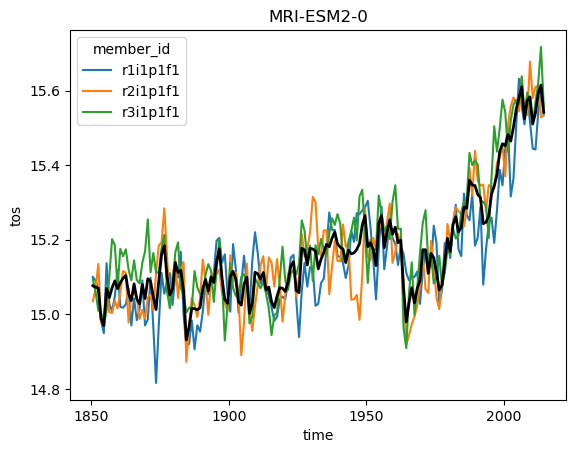
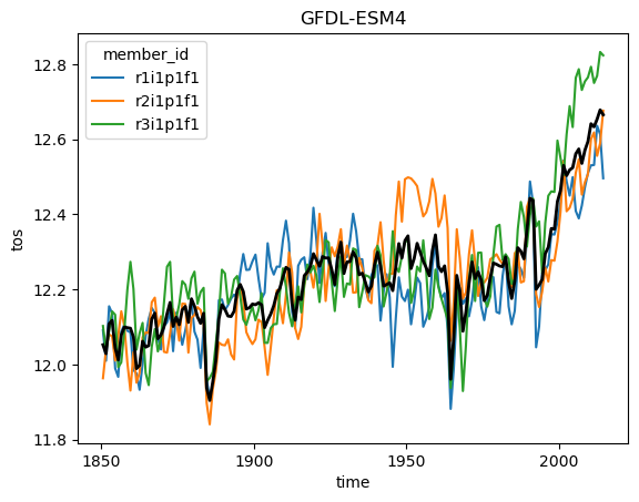
Ok but now lets analyze the data! Using what we know about xarray we can get a timeseries of the global sea surface temperature:

for name, ds in ddict.items():
    # construct yearly global mean timeseries
    mean_temp = ds.tos.mean(['x', 'y']).coarsen(time=12).mean()
    plt.figure()
    mean_temp.plot(hue='member_id')
    # lets also plot the average over all members
    mean_temp.mean('member_id').plot(color='k', linewidth=2)
    plt.title(ds.attrs['source_id']) #Extract the model name right from the dataset metadata
    plt.show()

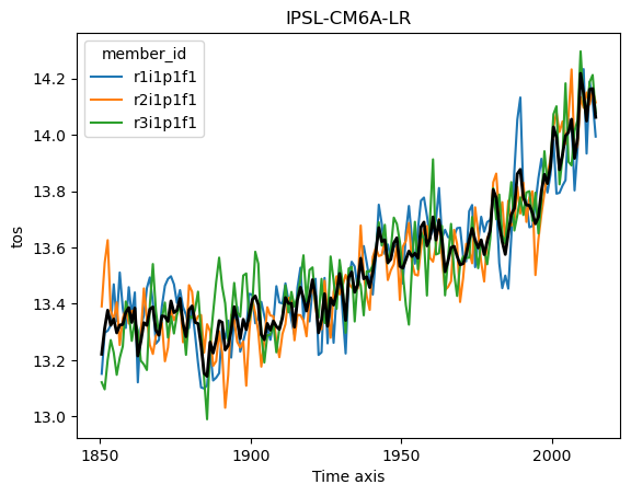
The above result is roughly correct, but as discussed in earlier lectures we need to do proper area weighting to ensure that different parts of the globe are weighted properly. You can look at the original notebook to see how to do things correctly.

Other ideas to explore:

• ESMs are not always on simple or similar grids:

  • For intercomparison, the most common choice is to regrid everything to a common grid. There is a package called xesmf for this. See this example.

  • Sometimes one needs to work with the native grid, and there is a package called xgcm for this. See this example.

• Datasets can sometimes (often) get quite big, making it challenging even for the largest computers to handle their analysis. One solution to this is to use multiple computers in parallel. There are a few different Python frameworks to do this, where dask is probably the most adopted framework at this point. See this example. One advantage to dask is that integrates natively with xarray, and with some forethought much of the parallelization can take place automatically.