Xarray Fundamentals#
Xarray data structures#
Like Pandas, xarray has two fundamental data structures:
a
DataArray, which holds a single multi-dimensional variable and its coordinatesa
Dataset, which holds multiple variables that potentially share the same coordinates
DataArray#
A DataArray has four essential attributes:
values: anumpy.ndarrayholding the array’s valuesdims: dimension names for each axis (e.g.,('x', 'y', 'z'))coords: a dict-like container of arrays (coordinates) that label each point (e.g., 1-dimensional arrays of numbers, datetime objects or strings)attrs: anOrderedDictto hold arbitrary metadata (attributes)
Let’s start by constructing some DataArrays manually
import numpy as np
import xarray as xr
from matplotlib import pyplot as plt
%matplotlib inline
plt.rcParams['figure.figsize'] = (8,5)
A simple DataArray without dimensions or coordinates isn’t much use.
da = xr.DataArray([9, 0, 2, 1, 0])
da
<xarray.DataArray (dim_0: 5)> Size: 40B
array([9, 0, 2, 1, 0])
Dimensions without coordinates: dim_0
We can add a dimension name…
da = xr.DataArray([9, 0, 2, 1, 0], dims=['x'])
da
<xarray.DataArray (x: 5)> Size: 40B
array([9, 0, 2, 1, 0])
Dimensions without coordinates: x
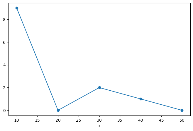
But things get most interesting when we add a coordinate:
da = xr.DataArray([9, 0, 2, 1, 0],
                  dims=['x'],
                  coords={'x': [10, 20, 30, 40, 50]})
da
<xarray.DataArray (x: 5)> Size: 40B
array([9, 0, 2, 1, 0])
Coordinates:
  * x        (x) int64 40B 10 20 30 40 50
This coordinate has been used to create an index, which works very similar to a Pandas index. In fact, under the hood, Xarray just reuses Pandas indexes.
da.indexes
Indexes:
    x        Index([10, 20, 30, 40, 50], dtype='int64', name='x')
Xarray has built-in plotting, like pandas.
da.plot(marker='o')
[<matplotlib.lines.Line2D at 0x79970a3cc5c0>]
Multidimensional DataArray#
If we are just dealing with 1D data, Pandas and Xarray have very similar capabilities. Xarray’s real potential comes with multidimensional data.
Let’s go back to the multidimensional ARGO data we loaded in the numpy lesson.
import pooch
url = "https://github.com/earth-DS-ML/summer_2025/raw/refs/heads/main/assignments/more_matplotlib_data/argo_data_example.zip"
files = pooch.retrieve(url, processor=pooch.Unzip(), known_hash="650948c4b84690d370ad6f8aa9279c165f5302d3d9a7d330d3c0232b9d244e13")
files.sort()
files
['/home/jovyan/.cache/pooch/e5b1bf9306e8d5b2c2efc5fa6b248fb0-argo_data_example.zip.unzip/argo_data_example/date.npy',
 '/home/jovyan/.cache/pooch/e5b1bf9306e8d5b2c2efc5fa6b248fb0-argo_data_example.zip.unzip/argo_data_example/latitude.npy',
 '/home/jovyan/.cache/pooch/e5b1bf9306e8d5b2c2efc5fa6b248fb0-argo_data_example.zip.unzip/argo_data_example/levels.npy',
 '/home/jovyan/.cache/pooch/e5b1bf9306e8d5b2c2efc5fa6b248fb0-argo_data_example.zip.unzip/argo_data_example/longitude.npy',
 '/home/jovyan/.cache/pooch/e5b1bf9306e8d5b2c2efc5fa6b248fb0-argo_data_example.zip.unzip/argo_data_example/pressure.npy',
 '/home/jovyan/.cache/pooch/e5b1bf9306e8d5b2c2efc5fa6b248fb0-argo_data_example.zip.unzip/argo_data_example/salinity.npy',
 '/home/jovyan/.cache/pooch/e5b1bf9306e8d5b2c2efc5fa6b248fb0-argo_data_example.zip.unzip/argo_data_example/temperature.npy']
We will manually load each of these variables into a numpy array. If this seems repetitive and inefficient, that’s the point! NumPy itself is not meant for managing groups of inter-related arrays. That’s what Xarray is for!
P = np.load(files[4]).T
S = np.load(files[5]).T
T = np.load(files[6]).T
date = np.load(files[0])
lat = np.load(files[1])
levels = np.load(files[2])
lon = np.load(files[3])
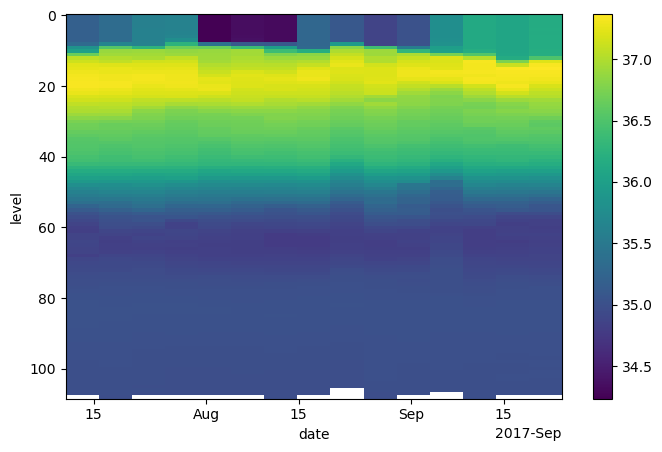
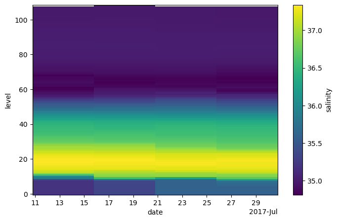
Let’s organize the data and coordinates of the salinity variable into a DataArray.
da_salinity = xr.DataArray(S, dims=['level', 'date'],
                           coords={'level': levels,
                                   'date': date},)
da_salinity
<xarray.DataArray (level: 109, date: 15)> Size: 7kB
array([[35.179, 35.334, 35.594, ..., 36.126, 36.082, 36.157],
       [35.18 , 35.333, 35.594, ..., 36.128, 36.081, 36.155],
       [35.18 , 35.333, 35.594, ..., 36.13 , 36.081, 36.155],
       ...,
       [34.986, 34.985, 34.983, ..., 34.991, 34.99 , 34.991],
       [34.985, 34.983, 34.982, ..., 34.99 , 34.989, 34.989],
       [   nan, 34.98 ,    nan, ..., 34.989,    nan,    nan]],
      shape=(109, 15), dtype=float32)
Coordinates:
  * level    (level) int64 872B 0 1 2 3 4 5 6 7 ... 102 103 104 105 106 107 108
* date (date) datetime64[ns] 120B 2017-07-13T06:53:00 ... 2017-09-21T06...da_salinity.plot(yincrease=False)
<matplotlib.collections.QuadMesh at 0x79970a493cb0>
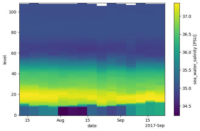
Attributes can be used to store metadata. What metadata should you store? The CF Conventions are a great resource for thinking about climate metadata. Below we define two of the required CF-conventions attributes.
da_salinity.attrs['units'] = 'PSU'
da_salinity.attrs['standard_name'] = 'sea_water_salinity'
da_salinity
<xarray.DataArray (level: 109, date: 15)> Size: 7kB
array([[35.179, 35.334, 35.594, ..., 36.126, 36.082, 36.157],
       [35.18 , 35.333, 35.594, ..., 36.128, 36.081, 36.155],
       [35.18 , 35.333, 35.594, ..., 36.13 , 36.081, 36.155],
       ...,
       [34.986, 34.985, 34.983, ..., 34.991, 34.99 , 34.991],
       [34.985, 34.983, 34.982, ..., 34.99 , 34.989, 34.989],
       [   nan, 34.98 ,    nan, ..., 34.989,    nan,    nan]],
      shape=(109, 15), dtype=float32)
Coordinates:
* level (level) int64 872B 0 1 2 3 4 5 6 7 ... 102 103 104 105 106 107 108
* date (date) datetime64[ns] 120B 2017-07-13T06:53:00 ... 2017-09-21T06...
Attributes:
units: PSU
standard_name: sea_water_salinityNow if we plot the data again, the name and units are automatically attached to the figure.
da_salinity.plot()
<matplotlib.collections.QuadMesh at 0x7997023684d0>
Datasets#
A Dataset holds many DataArrays which potentially can share coordinates. In analogy to pandas:
pandas.Series : pandas.Dataframe :: xarray.DataArray : xarray.Dataset
Constructing Datasets manually is a bit more involved in terms of syntax. The Dataset constructor takes three arguments:
data_varsshould be a dictionary with each key as the name of the variable and each value as one of:A
DataArrayor VariableA tuple of the form
(dims, data[, attrs]), which is converted into arguments for VariableA pandas object, which is converted into a
DataArrayA 1D array or list, which is interpreted as values for a one dimensional coordinate variable along the same dimension as it’s name
coordsshould be a dictionary of the same form as data_vars.attrsshould be a dictionary.
Let’s put together a Dataset with temperature, salinity and pressure all together
argo = xr.Dataset(
data_vars={
'salinity': (('level', 'date'), S),
'temperature': (('level', 'date'), T),
'pressure': (('level', 'date'), P)
},
coords={
'level': levels,
'date': date
}
)
argo
<xarray.Dataset> Size: 21kB
Dimensions: (level: 109, date: 15)
Coordinates:
* level (level) int64 872B 0 1 2 3 4 5 6 ... 103 104 105 106 107 108
* date (date) datetime64[ns] 120B 2017-07-13T06:53:00 ... 2017-09-2...
Data variables:
salinity (level, date) float32 7kB 35.18 35.33 35.59 ... 34.99 nan nan
temperature (level, date) float32 7kB 27.97 28.2 28.31 ... 3.688 nan nan
pressure (level, date) float32 7kB 3.0 3.0 3.0 3.0 ... 2.005e+03 nan nanWhat about lon and lat? We forgot them in the creation process, but we can add them after the fact.
argo.coords['lon'] = lon
argo
<xarray.Dataset> Size: 21kB
Dimensions: (level: 109, date: 15, lon: 15)
Coordinates:
* level (level) int64 872B 0 1 2 3 4 5 6 ... 103 104 105 106 107 108
* date (date) datetime64[ns] 120B 2017-07-13T06:53:00 ... 2017-09-2...
* lon (lon) float64 120B -59.99 -59.8 -59.7 ... -58.78 -58.75 -58.83
Data variables:
salinity (level, date) float32 7kB 35.18 35.33 35.59 ... 34.99 nan nan
temperature (level, date) float32 7kB 27.97 28.2 28.31 ... 3.688 nan nan
pressure (level, date) float32 7kB 3.0 3.0 3.0 3.0 ... 2.005e+03 nan nanThat was not quite right…we want lon to have dimension date:
del argo['lon']
argo.coords['lon'] = ('date', lon)
argo.coords['lat'] = ('date', lat)
argo
<xarray.Dataset> Size: 21kB
Dimensions: (level: 109, date: 15)
Coordinates:
* level (level) int64 872B 0 1 2 3 4 5 6 ... 103 104 105 106 107 108
* date (date) datetime64[ns] 120B 2017-07-13T06:53:00 ... 2017-09-2...
lon (date) float64 120B -59.99 -59.8 -59.7 ... -58.78 -58.75 -58.83
lat (date) float64 120B 20.21 20.16 19.92 ... 18.52 18.33 18.3
Data variables:
salinity (level, date) float32 7kB 35.18 35.33 35.59 ... 34.99 nan nan
temperature (level, date) float32 7kB 27.97 28.2 28.31 ... 3.688 nan nan
pressure (level, date) float32 7kB 3.0 3.0 3.0 3.0 ... 2.005e+03 nan nanCoordinates vs. Data Variables#
Data variables can be modified through arithmentic operations or other functions. Coordinates are always keept the same.
argo * 10000
<xarray.Dataset> Size: 21kB
Dimensions: (level: 109, date: 15)
Coordinates:
* level (level) int64 872B 0 1 2 3 4 5 6 ... 103 104 105 106 107 108
* date (date) datetime64[ns] 120B 2017-07-13T06:53:00 ... 2017-09-2...
lon (date) float64 120B -59.99 -59.8 -59.7 ... -58.78 -58.75 -58.83
lat (date) float64 120B 20.21 20.16 19.92 ... 18.52 18.33 18.3
Data variables:
salinity (level, date) float32 7kB 3.518e+05 3.533e+05 ... nan nan
temperature (level, date) float32 7kB 2.797e+05 2.82e+05 ... nan nan
pressure (level, date) float32 7kB 3e+04 3e+04 3e+04 ... nan nanargo
<xarray.Dataset> Size: 21kB
Dimensions: (level: 109, date: 15)
Coordinates:
* level (level) int64 872B 0 1 2 3 4 5 6 ... 103 104 105 106 107 108
* date (date) datetime64[ns] 120B 2017-07-13T06:53:00 ... 2017-09-2...
lon (date) float64 120B -59.99 -59.8 -59.7 ... -58.78 -58.75 -58.83
lat (date) float64 120B 20.21 20.16 19.92 ... 18.52 18.33 18.3
Data variables:
salinity (level, date) float32 7kB 35.18 35.33 35.59 ... 34.99 nan nan
temperature (level, date) float32 7kB 27.97 28.2 28.31 ... 3.688 nan nan
pressure (level, date) float32 7kB 3.0 3.0 3.0 3.0 ... 2.005e+03 nan nanprint(argo)
<xarray.Dataset> Size: 21kB
Dimensions: (level: 109, date: 15)
Coordinates:
* level (level) int64 872B 0 1 2 3 4 5 6 ... 103 104 105 106 107 108
* date (date) datetime64[ns] 120B 2017-07-13T06:53:00 ... 2017-09-2...
lon (date) float64 120B -59.99 -59.8 -59.7 ... -58.78 -58.75 -58.83
lat (date) float64 120B 20.21 20.16 19.92 ... 18.52 18.33 18.3
Data variables:
salinity (level, date) float32 7kB 35.18 35.33 35.59 ... 34.99 nan nan
temperature (level, date) float32 7kB 27.97 28.2 28.31 ... 3.688 nan nan
pressure (level, date) float32 7kB 3.0 3.0 3.0 3.0 ... 2.005e+03 nan nan
The * symbol in the representation above indicates that level and date are “dimension coordinates” (they describe the coordinates associated with data variable axes) while lon and lat are “non-dimension coordinates”. We can make any variable a non-dimension coordiante.
Selecting Data (Indexing)#
We can always use regular numpy indexing and slicing on DataArrays
argo.salinity[2]
<xarray.DataArray 'salinity' (date: 15)> Size: 60B
array([35.18 , 35.333, 35.594, 35.607, 34.236, 34.345, 34.311, 35.272,
35.086, 34.863, 35.026, 35.773, 36.13 , 36.081, 36.155],
dtype=float32)
Coordinates:
level int64 8B 2
* date (date) datetime64[ns] 120B 2017-07-13T06:53:00 ... 2017-09-21T06...
lon (date) float64 120B -59.99 -59.8 -59.7 ... -58.78 -58.75 -58.83
lat (date) float64 120B 20.21 20.16 19.92 19.65 ... 18.52 18.33 18.3argo.salinity[2].plot()
[<matplotlib.lines.Line2D at 0x79970224d1c0>]
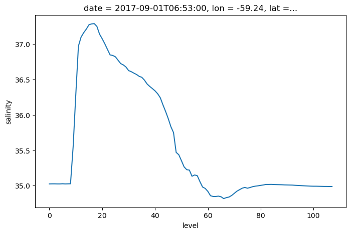
argo.salinity[:, 10]
<xarray.DataArray 'salinity' (level: 109)> Size: 436B
array([35.025, 35.026, 35.026, 35.025, 35.025, 35.027, 35.025, 35.026,
35.027, 35.55 , 36.282, 36.972, 37.099, 37.162, 37.213, 37.274,
37.286, 37.29 , 37.25 , 37.141, 37.076, 37.004, 36.925, 36.847,
36.84 , 36.821, 36.773, 36.725, 36.706, 36.677, 36.626, 36.611,
36.59 , 36.571, 36.545, 36.531, 36.491, 36.437, 36.402, 36.372,
36.34 , 36.299, 36.242, 36.142, 36.049, 35.948, 35.834, 35.75 ,
35.47 , 35.437, 35.353, 35.266, 35.226, 35.22 , 35.133, 35.151,
35.141, 35.057, 34.981, 34.961, 34.919, 34.858, 34.847, 34.847,
34.852, 34.843, 34.817, 34.831, 34.839, 34.861, 34.891, 34.922,
34.943, 34.964, 34.975, 34.964, 34.974, 34.986, 34.993, 34.998,
35.004, 35.01 , 35.017, 35.017, 35.018, 35.016, 35.015, 35.014,
35.013, 35.011, 35.01 , 35.009, 35.008, 35.005, 35.003, 35.001,
34.999, 34.997, 34.995, 34.993, 34.992, 34.992, 34.991, 34.99 ,
34.989, 34.989, 34.988, 34.988, nan], dtype=float32)
Coordinates:
* level (level) int64 872B 0 1 2 3 4 5 6 7 ... 102 103 104 105 106 107 108
date datetime64[ns] 8B 2017-09-01T06:53:00
lon float64 8B -59.24
lat float64 8B 18.8argo.salinity[:, 10].plot()
[<matplotlib.lines.Line2D at 0x7997020c6960>]
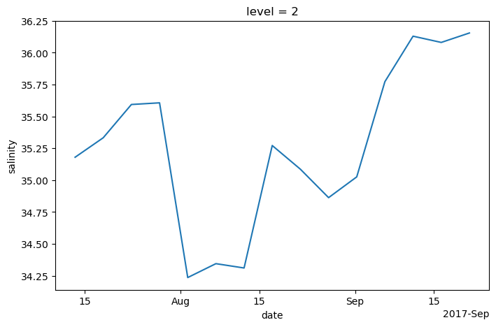
However, it is often much more powerful to use xarray’s .sel() method to use label-based indexing.
argo.salinity.sel(level=2)
<xarray.DataArray 'salinity' (date: 15)> Size: 60B
array([35.18 , 35.333, 35.594, 35.607, 34.236, 34.345, 34.311, 35.272,
35.086, 34.863, 35.026, 35.773, 36.13 , 36.081, 36.155],
dtype=float32)
Coordinates:
level int64 8B 2
* date (date) datetime64[ns] 120B 2017-07-13T06:53:00 ... 2017-09-21T06...
lon (date) float64 120B -59.99 -59.8 -59.7 ... -58.78 -58.75 -58.83
lat (date) float64 120B 20.21 20.16 19.92 19.65 ... 18.52 18.33 18.3argo.salinity.sel(level=2).plot()
[<matplotlib.lines.Line2D at 0x799702158770>]
argo.date
<xarray.DataArray 'date' (date: 15)> Size: 120B
array(['2017-07-13T06:53:00.000000000', '2017-07-18T06:49:00.000000000',
       '2017-07-23T06:49:00.000000000', '2017-07-28T06:47:00.000000000',
       '2017-08-02T06:49:00.000000000', '2017-08-07T06:50:00.000000000',
       '2017-08-12T06:53:00.000000000', '2017-08-17T06:52:00.000000000',
       '2017-08-22T06:55:00.000000000', '2017-08-27T06:57:00.000000000',
       '2017-09-01T06:53:00.000000000', '2017-09-06T06:48:00.000000000',
       '2017-09-11T06:49:00.000000000', '2017-09-16T06:55:00.000000000',
       '2017-09-21T06:52:00.000000000'], dtype='datetime64[ns]')
Coordinates:
* date (date) datetime64[ns] 120B 2017-07-13T06:53:00 ... 2017-09-21T06...
lon (date) float64 120B -59.99 -59.8 -59.7 ... -58.78 -58.75 -58.83
lat (date) float64 120B 20.21 20.16 19.92 19.65 ... 18.52 18.33 18.3argo.salinity.sel(date='2017-07-23')
<xarray.DataArray 'salinity' (level: 109, date: 1)> Size: 436B
array([[35.594],
[35.594],
[35.594],
[35.593],
[35.597],
[35.596],
[35.601],
[35.6 ],
[35.609],
[36.258],
[36.895],
[36.93 ],
[36.973],
[37.138],
[37.222],
[37.238],
[37.272],
[37.311],
[37.315],
[37.298],
...
[35.01 ],
[35.007],
[35.004],
[35.003],
[34.999],
[34.997],
[34.994],
[34.993],
[34.991],
[34.99 ],
[34.99 ],
[34.989],
[34.987],
[34.984],
[34.983],
[34.983],
[34.982],
[34.983],
[34.982],
[ nan]], dtype=float32)
Coordinates:
* level (level) int64 872B 0 1 2 3 4 5 6 7 ... 102 103 104 105 106 107 108
* date (date) datetime64[ns] 8B 2017-07-23T06:49:00
lon (date) float64 8B -59.7
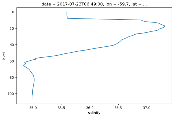
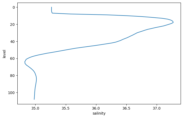
lat (date) float64 8B 19.92argo.salinity.sel(date='2017-07-23').plot(y='level', yincrease=False)
[<matplotlib.lines.Line2D at 0x799701fd02c0>]
.sel() also supports slicing. Unfortunately we have to use a somewhat awkward syntax, but it still works.
argo.salinity.sel(date=slice('2017-07-01', '2017-08-01'))
<xarray.DataArray 'salinity' (level: 109, date: 4)> Size: 2kB
array([[35.179, 35.334, 35.594, 35.609],
       [35.18 , 35.333, 35.594, 35.608],
       [35.18 , 35.333, 35.594, 35.607],
       [35.18 , 35.333, 35.593, 35.607],
       [35.179, 35.333, 35.597, 35.612],
       [35.18 , 35.334, 35.596, 35.64 ],
       [35.18 , 35.333, 35.601, 35.665],
       [35.18 , 35.336, 35.6  , 35.766],
       [35.309, 35.661, 35.609, 36.262],
       [35.831, 36.531, 36.258, 36.676],
       [36.008, 36.88 , 36.895, 36.859],
       [36.649, 36.926, 36.93 , 36.895],
       [37.063, 37.008, 36.973, 37.065],
       [37.132, 37.068, 37.138, 37.16 ],
       [37.223, 37.214, 37.222, 37.216],
       [37.255, 37.262, 37.238, 37.251],
       [37.287, 37.264, 37.272, 37.279],
       [37.311, 37.296, 37.311, 37.287],
       [37.324, 37.301, 37.315, 37.288],
       [37.333, 37.325, 37.298, 37.302],
...
       [35.019, 35.015, 35.01 , 35.01 ],
       [35.017, 35.013, 35.007, 35.008],
       [35.013, 35.01 , 35.004, 35.005],
       [35.009, 35.008, 35.003, 35.002],
       [35.005, 35.005, 34.999, 34.998],
       [35.003, 35.003, 34.997, 34.994],
       [35.001, 35.001, 34.994, 34.992],
       [34.999, 34.999, 34.993, 34.99 ],
       [34.996, 34.998, 34.991, 34.988],
       [34.993, 34.997, 34.99 , 34.985],
       [34.991, 34.995, 34.99 , 34.984],
       [34.989, 34.992, 34.989, 34.981],
       [34.989, 34.991, 34.987, 34.98 ],
       [34.991, 34.989, 34.984, 34.979],
       [34.99 , 34.989, 34.983, 34.979],
       [34.988, 34.988, 34.983, 34.977],
       [34.986, 34.987, 34.982, 34.975],
       [34.986, 34.985, 34.983, 34.974],
       [34.985, 34.983, 34.982, 34.973],
       [   nan, 34.98 ,    nan,    nan]], dtype=float32)
Coordinates:
  * level    (level) int64 872B 0 1 2 3 4 5 6 7 ... 102 103 104 105 106 107 108
  * date     (date) datetime64[ns] 32B 2017-07-13T06:53:00 ... 2017-07-28T06:...
    lon      (date) float64 32B -59.99 -59.8 -59.7 -59.72
lat (date) float64 32B 20.21 20.16 19.92 19.65argo.salinity.sel(date=slice('2017-07-01', '2017-08-01')).plot()
<matplotlib.collections.QuadMesh at 0x7997020c4e00>
.sel() also works on the whole Dataset
argo.sel(date='2017-07-23')
<xarray.Dataset> Size: 2kB
Dimensions:      (level: 109, date: 1)
Coordinates:
  * level        (level) int64 872B 0 1 2 3 4 5 6 ... 103 104 105 106 107 108
  * date         (date) datetime64[ns] 8B 2017-07-23T06:49:00
    lon          (date) float64 8B -59.7
    lat          (date) float64 8B 19.92
Data variables:
    salinity     (level, date) float32 436B 35.59 35.59 35.59 ... 34.98 nan
    temperature  (level, date) float32 436B 28.31 28.31 28.31 ... 3.699 nan
pressure (level, date) float32 436B 3.0 4.0 5.0 ... 1.983e+03 nanComputation#
Xarray dataarrays and datasets work seamlessly with arithmetic operators and numpy array functions.
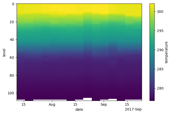
temp_kelvin = argo.temperature + 273.15
temp_kelvin.plot(yincrease=False)
<matplotlib.collections.QuadMesh at 0x79970223ad80>
We can also combine multiple xarray datasets in arithemtic operations
g = 9.8
buoyancy = g * (2e-4 * argo.temperature - 7e-4 * argo.salinity)
buoyancy.plot(yincrease=False)
<matplotlib.collections.QuadMesh at 0x799702193740>
Broadcasting, Aligment, and Combining Data#
Broadcasting#
Broadcasting arrays in numpy is a nightmare. It is much easier when the data axes are labeled!
This is a useless calculation, but it illustrates how perfoming an operation on arrays with differenty coordinates will result in automatic broadcasting
level_times_lat = argo.level * argo.lat
level_times_lat
<xarray.DataArray (level: 109, date: 15)> Size: 13kB
array([[   0.   ,    0.   ,    0.   , ...,    0.   ,    0.   ,    0.   ],
       [  20.212,   20.16 ,   19.923, ...,   18.515,   18.332,   18.298],
       [  40.424,   40.32 ,   39.846, ...,   37.03 ,   36.664,   36.596],
       ...,
       [2142.472, 2136.96 , 2111.838, ..., 1962.59 , 1943.192, 1939.588],
       [2162.684, 2157.12 , 2131.761, ..., 1981.105, 1961.524, 1957.886],
       [2182.896, 2177.28 , 2151.684, ..., 1999.62 , 1979.856, 1976.184]],
      shape=(109, 15))
Coordinates:
  * level    (level) int64 872B 0 1 2 3 4 5 6 7 ... 102 103 104 105 106 107 108
  * date     (date) datetime64[ns] 120B 2017-07-13T06:53:00 ... 2017-09-21T06...
    lon      (date) float64 120B -59.99 -59.8 -59.7 ... -58.78 -58.75 -58.83
lat (date) float64 120B 20.21 20.16 19.92 19.65 ... 18.52 18.33 18.3level_times_lat.plot()
<matplotlib.collections.QuadMesh at 0x799701e0e810>
Alignment#
If you try to perform operations on DataArrays that share a dimension name, Xarray will try to align them first. This works nearly identically to Pandas, except that there can be multiple dimensions to align over.
To see how alignment works, we will create some subsets of our original data.
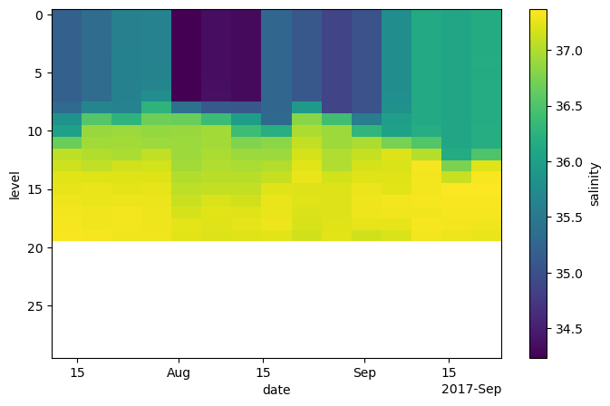
argo.salinity.isel(level=slice(0, 30)).plot(yincrease=False)
<matplotlib.collections.QuadMesh at 0x799701f31d30>
sa_surf = argo.salinity.isel(level=slice(0, 20))
sa_mid = argo.salinity.isel(level=slice(10, 30))
sa_surf
<xarray.DataArray 'salinity' (level: 20, date: 15)> Size: 1kB
array([[35.179, 35.334, 35.594, 35.609, 34.238, 34.342, 34.312, 35.272,
        35.086, 34.864, 35.025, 35.776, 36.126, 36.082, 36.157],
       [35.18 , 35.333, 35.594, 35.608, 34.237, 34.345, 34.311, 35.272,
        35.085, 34.863, 35.026, 35.774, 36.128, 36.081, 36.155],
       [35.18 , 35.333, 35.594, 35.607, 34.236, 34.345, 34.311, 35.272,
        35.086, 34.863, 35.026, 35.773, 36.13 , 36.081, 36.155],
       [35.18 , 35.333, 35.593, 35.607, 34.236, 34.343, 34.312, 35.271,
        35.087, 34.863, 35.025, 35.771, 36.129, 36.082, 36.156],
       [35.179, 35.333, 35.597, 35.612, 34.237, 34.343, 34.31 , 35.272,
        35.086, 34.862, 35.025, 35.769, 36.129, 36.082, 36.159],
       [35.18 , 35.334, 35.596, 35.64 , 34.237, 34.342, 34.312, 35.272,
        35.086, 34.861, 35.027, 35.769, 36.128, 36.082, 36.156],
       [35.18 , 35.333, 35.601, 35.665, 34.237, 34.353, 34.312, 35.272,
        35.086, 34.863, 35.025, 35.77 , 36.128, 36.083, 36.159],
       [35.18 , 35.336, 35.6  , 35.766, 34.238, 34.36 , 34.311, 35.272,
        35.088, 34.863, 35.026, 35.782, 36.127, 36.083, 36.159],
       [35.309, 35.661, 35.609, 36.262, 35.393, 35.113, 35.081, 35.275,
        35.937, 34.862, 35.027, 35.809, 36.127, 36.082, 36.158],
       [35.831, 36.531, 36.258, 36.676, 36.648, 36.366, 35.962, 35.299,
        36.807, 36.407, 35.55 , 35.978, 36.127, 36.082, 36.167],
...
        36.981, 36.912, 36.282, 36.019, 36.175, 36.083, 36.18 ],
       [36.649, 36.926, 36.93 , 36.895, 36.897, 36.938, 36.762, 36.829,
        37.078, 36.915, 36.972, 36.721, 36.521, 36.086, 36.189],
       [37.063, 37.008, 36.973, 37.065, 36.904, 36.977, 36.893, 36.898,
        37.171, 36.99 , 37.099, 37.2  , 37.022, 36.156, 36.494],
       [37.132, 37.068, 37.138, 37.16 , 36.935, 36.998, 36.968, 37.002,
        37.231, 36.996, 37.162, 37.189, 37.323, 36.749, 37.22 ],
       [37.223, 37.214, 37.222, 37.216, 37.004, 37.05 , 37.032, 37.096,
        37.269, 37.149, 37.213, 37.222, 37.31 , 37.102, 37.341],
       [37.255, 37.262, 37.238, 37.251, 37.06 , 37.087, 37.085, 37.215,
        37.209, 37.208, 37.274, 37.223, 37.315, 37.356, 37.369],
       [37.287, 37.264, 37.272, 37.279, 37.105, 37.194, 37.143, 37.266,
        37.213, 37.209, 37.286, 37.32 , 37.323, 37.338, 37.334],
       [37.311, 37.296, 37.311, 37.287, 37.17 , 37.231, 37.212, 37.269,
        37.186, 37.206, 37.29 , 37.3  , 37.302, 37.327, 37.326],
       [37.324, 37.301, 37.315, 37.288, 37.239, 37.222, 37.236, 37.284,
        37.179, 37.212, 37.25 , 37.257, 37.33 , 37.319, 37.305],
       [37.333, 37.325, 37.298, 37.302, 37.233, 37.205, 37.211, 37.228,
        37.139, 37.224, 37.141, 37.189, 37.312, 37.285, 37.261]],
      dtype=float32)
Coordinates:
  * level    (level) int64 160B 0 1 2 3 4 5 6 7 8 ... 11 12 13 14 15 16 17 18 19
  * date     (date) datetime64[ns] 120B 2017-07-13T06:53:00 ... 2017-09-21T06...
    lon      (date) float64 120B -59.99 -59.8 -59.7 ... -58.78 -58.75 -58.83
lat (date) float64 120B 20.21 20.16 19.92 19.65 ... 18.52 18.33 18.3By default, when we combine multiple arrays in mathematical operations, Xarray performs an “inner join”.
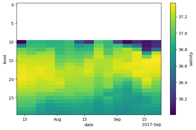
(sa_surf * sa_mid).level
<xarray.DataArray 'level' (level: 10)> Size: 80B
array([10, 11, 12, 13, 14, 15, 16, 17, 18, 19])
Coordinates:
  * level    (level) int64 80B 10 11 12 13 14 15 16 17 18 19
(sa_surf * sa_mid).plot(yincrease=False)
<matplotlib.collections.QuadMesh at 0x799701de8ce0>
We can override this behavior by manually aligning the data
sa_surf_outer, sa_mid_outer = xr.align(sa_surf, sa_mid, join='outer')
sa_surf_outer.level
<xarray.DataArray 'level' (level: 30)> Size: 240B
array([ 0,  1,  2,  3,  4,  5,  6,  7,  8,  9, 10, 11, 12, 13, 14, 15, 16, 17,
       18, 19, 20, 21, 22, 23, 24, 25, 26, 27, 28, 29])
Coordinates:
* level (level) int64 240B 0 1 2 3 4 5 6 7 8 ... 21 22 23 24 25 26 27 28 29As we can see, missing data (NaNs) have been filled in where the array was extended.
sa_surf_outer.plot(yincrease=False)
<matplotlib.collections.QuadMesh at 0x799701d82360>
sa_mid_outer.plot(yincrease=False)
<matplotlib.collections.QuadMesh at 0x799701ac5c10>
We can also use join='right' and join='left'.
Combing Data: Concat and Merge#
The ability to combine many smaller arrays into a single big Dataset is one of the main advantages of Xarray. To take advantage of this, we need to learn two operations that help us combine data:
xr.contact: to concatenate multiple arrays into one bigger array along their dimensionsxr.merge: to combine multiple different arrays into a dataset
First let’s look at concat. Let’s re-combine the subsetted data from the previous step.
sa_surf_mid = xr.concat([sa_surf, sa_mid], dim='level')
sa_surf_mid
<xarray.DataArray 'salinity' (level: 40, date: 15)> Size: 2kB
array([[35.179, 35.334, 35.594, 35.609, 34.238, 34.342, 34.312, 35.272,
        35.086, 34.864, 35.025, 35.776, 36.126, 36.082, 36.157],
       [35.18 , 35.333, 35.594, 35.608, 34.237, 34.345, 34.311, 35.272,
        35.085, 34.863, 35.026, 35.774, 36.128, 36.081, 36.155],
       [35.18 , 35.333, 35.594, 35.607, 34.236, 34.345, 34.311, 35.272,
        35.086, 34.863, 35.026, 35.773, 36.13 , 36.081, 36.155],
       [35.18 , 35.333, 35.593, 35.607, 34.236, 34.343, 34.312, 35.271,
        35.087, 34.863, 35.025, 35.771, 36.129, 36.082, 36.156],
       [35.179, 35.333, 35.597, 35.612, 34.237, 34.343, 34.31 , 35.272,
        35.086, 34.862, 35.025, 35.769, 36.129, 36.082, 36.159],
       [35.18 , 35.334, 35.596, 35.64 , 34.237, 34.342, 34.312, 35.272,
        35.086, 34.861, 35.027, 35.769, 36.128, 36.082, 36.156],
       [35.18 , 35.333, 35.601, 35.665, 34.237, 34.353, 34.312, 35.272,
        35.086, 34.863, 35.025, 35.77 , 36.128, 36.083, 36.159],
       [35.18 , 35.336, 35.6  , 35.766, 34.238, 34.36 , 34.311, 35.272,
        35.088, 34.863, 35.026, 35.782, 36.127, 36.083, 36.159],
       [35.309, 35.661, 35.609, 36.262, 35.393, 35.113, 35.081, 35.275,
        35.937, 34.862, 35.027, 35.809, 36.127, 36.082, 36.158],
       [35.831, 36.531, 36.258, 36.676, 36.648, 36.366, 35.962, 35.299,
        36.807, 36.407, 35.55 , 35.978, 36.127, 36.082, 36.167],
...
        37.09 , 37.149, 37.076, 37.038, 37.149, 37.326, 37.178],
       [37.299, 37.279, 37.223, 37.244, 37.274, 37.158, 37.176, 37.155,
        37.086, 37.135, 37.004, 36.902, 37.06 , 37.265, 37.113],
       [37.267, 37.245, 37.206, 37.208, 37.208, 37.129, 37.127, 37.136,
        37.044, 37.115, 36.925, 36.83 , 37.   , 37.159, 37.057],
       [37.194, 37.185, 37.167, 37.184, 37.127, 37.108, 37.095, 37.094,
        36.995, 36.931, 36.847, 36.759, 36.912, 37.031, 37.016],
       [37.144, 37.13 , 37.075, 37.062, 37.049, 37.076, 37.013, 37.03 ,
        36.939, 36.819, 36.84 , 36.778, 36.81 , 36.903, 36.925],
       [37.075, 37.053, 37.016, 36.956, 36.966, 36.99 , 36.963, 36.934,
        36.846, 36.928, 36.821, 36.76 , 36.732, 36.797, 36.875],
       [37.007, 37.022, 36.939, 36.833, 36.89 , 36.892, 36.892, 36.852,
        36.759, 36.85 , 36.773, 36.717, 36.705, 36.762, 36.854],
       [36.987, 36.97 , 36.821, 36.752, 36.8  , 36.829, 36.822, 36.798,
        36.729, 36.783, 36.725, 36.692, 36.748, 36.796, 36.811],
       [36.908, 36.905, 36.778, 36.731, 36.73 , 36.763, 36.772, 36.78 ,
        36.708, 36.759, 36.706, 36.669, 36.729, 36.753, 36.76 ],
       [36.824, 36.817, 36.754, 36.693, 36.697, 36.705, 36.772, 36.746,
        36.682, 36.716, 36.677, 36.646, 36.691, 36.701, 36.673]],
      dtype=float32)
Coordinates:
  * level    (level) int64 320B 0 1 2 3 4 5 6 7 8 ... 21 22 23 24 25 26 27 28 29
  * date     (date) datetime64[ns] 120B 2017-07-13T06:53:00 ... 2017-09-21T06...
    lon      (date) float64 120B -59.99 -59.8 -59.7 ... -58.78 -58.75 -58.83
lat (date) float64 120B 20.21 20.16 19.92 19.65 ... 18.52 18.33 18.3Warning
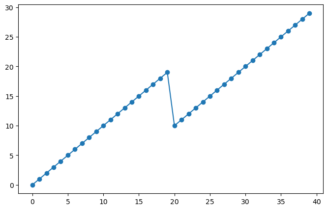
Xarray won’t check the values of the coordinates before concat. It will just stick everything together into a new array.
In this case, we had overlapping data. We can see this by looking at the level coordinate.
sa_surf_mid.level
<xarray.DataArray 'level' (level: 40)> Size: 320B
array([ 0,  1,  2,  3,  4,  5,  6,  7,  8,  9, 10, 11, 12, 13, 14, 15, 16, 17,
       18, 19, 10, 11, 12, 13, 14, 15, 16, 17, 18, 19, 20, 21, 22, 23, 24, 25,
       26, 27, 28, 29])
Coordinates:
* level (level) int64 320B 0 1 2 3 4 5 6 7 8 ... 21 22 23 24 25 26 27 28 29plt.plot(sa_surf_mid.level.values, marker='o')
[<matplotlib.lines.Line2D at 0x799701d4ddc0>]
We can also concat data along a new dimension, e.g.
sa_concat_new = xr.concat([sa_surf, sa_mid], dim='newdim')
sa_concat_new
<xarray.DataArray 'salinity' (newdim: 2, level: 30, date: 15)> Size: 4kB
array([[[35.179, 35.334, 35.594, 35.609, 34.238, 34.342, 34.312, 35.272,
         35.086, 34.864, 35.025, 35.776, 36.126, 36.082, 36.157],
        [35.18 , 35.333, 35.594, 35.608, 34.237, 34.345, 34.311, 35.272,
         35.085, 34.863, 35.026, 35.774, 36.128, 36.081, 36.155],
        [35.18 , 35.333, 35.594, 35.607, 34.236, 34.345, 34.311, 35.272,
         35.086, 34.863, 35.026, 35.773, 36.13 , 36.081, 36.155],
        [35.18 , 35.333, 35.593, 35.607, 34.236, 34.343, 34.312, 35.271,
         35.087, 34.863, 35.025, 35.771, 36.129, 36.082, 36.156],
        [35.179, 35.333, 35.597, 35.612, 34.237, 34.343, 34.31 , 35.272,
         35.086, 34.862, 35.025, 35.769, 36.129, 36.082, 36.159],
        [35.18 , 35.334, 35.596, 35.64 , 34.237, 34.342, 34.312, 35.272,
         35.086, 34.861, 35.027, 35.769, 36.128, 36.082, 36.156],
        [35.18 , 35.333, 35.601, 35.665, 34.237, 34.353, 34.312, 35.272,
         35.086, 34.863, 35.025, 35.77 , 36.128, 36.083, 36.159],
        [35.18 , 35.336, 35.6  , 35.766, 34.238, 34.36 , 34.311, 35.272,
         35.088, 34.863, 35.026, 35.782, 36.127, 36.083, 36.159],
        [35.309, 35.661, 35.609, 36.262, 35.393, 35.113, 35.081, 35.275,
         35.937, 34.862, 35.027, 35.809, 36.127, 36.082, 36.158],
        [35.831, 36.531, 36.258, 36.676, 36.648, 36.366, 35.962, 35.299,
         36.807, 36.407, 35.55 , 35.978, 36.127, 36.082, 36.167],
...
         37.09 , 37.149, 37.076, 37.038, 37.149, 37.326, 37.178],
        [37.299, 37.279, 37.223, 37.244, 37.274, 37.158, 37.176, 37.155,
         37.086, 37.135, 37.004, 36.902, 37.06 , 37.265, 37.113],
        [37.267, 37.245, 37.206, 37.208, 37.208, 37.129, 37.127, 37.136,
         37.044, 37.115, 36.925, 36.83 , 37.   , 37.159, 37.057],
        [37.194, 37.185, 37.167, 37.184, 37.127, 37.108, 37.095, 37.094,
         36.995, 36.931, 36.847, 36.759, 36.912, 37.031, 37.016],
        [37.144, 37.13 , 37.075, 37.062, 37.049, 37.076, 37.013, 37.03 ,
         36.939, 36.819, 36.84 , 36.778, 36.81 , 36.903, 36.925],
        [37.075, 37.053, 37.016, 36.956, 36.966, 36.99 , 36.963, 36.934,
         36.846, 36.928, 36.821, 36.76 , 36.732, 36.797, 36.875],
        [37.007, 37.022, 36.939, 36.833, 36.89 , 36.892, 36.892, 36.852,
         36.759, 36.85 , 36.773, 36.717, 36.705, 36.762, 36.854],
        [36.987, 36.97 , 36.821, 36.752, 36.8  , 36.829, 36.822, 36.798,
         36.729, 36.783, 36.725, 36.692, 36.748, 36.796, 36.811],
        [36.908, 36.905, 36.778, 36.731, 36.73 , 36.763, 36.772, 36.78 ,
         36.708, 36.759, 36.706, 36.669, 36.729, 36.753, 36.76 ],
        [36.824, 36.817, 36.754, 36.693, 36.697, 36.705, 36.772, 36.746,
         36.682, 36.716, 36.677, 36.646, 36.691, 36.701, 36.673]]],
      dtype=float32)
Coordinates:
  * level    (level) int64 240B 0 1 2 3 4 5 6 7 8 ... 21 22 23 24 25 26 27 28 29
  * date     (date) datetime64[ns] 120B 2017-07-13T06:53:00 ... 2017-09-21T06...
    lon      (date) float64 120B -59.99 -59.8 -59.7 ... -58.78 -58.75 -58.83
    lat      (date) float64 120B 20.21 20.16 19.92 19.65 ... 18.52 18.33 18.3
Dimensions without coordinates: newdimplt.figure(figsize=(12, 4))
plt.subplot(121)
sa_concat_new.isel(newdim=0).plot()
plt.subplot(122)
sa_concat_new.isel(newdim=1).plot()
plt.tight_layout()
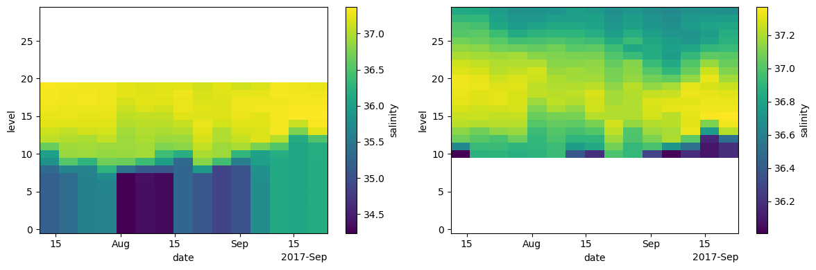
Note that the data were aligned using an outer join along the non-concat dimensions.
Instead of specifying a new dimension name, we can pass a new Pandas index object explicitly to concat.
This will create a new dimension coordinate and corresponding index.
We can merge both DataArrays and Datasets.
xr.merge([argo.salinity, argo.temperature])
<xarray.Dataset> Size: 14kB
Dimensions:      (level: 109, date: 15)
Coordinates:
  * level        (level) int64 872B 0 1 2 3 4 5 6 ... 103 104 105 106 107 108
  * date         (date) datetime64[ns] 120B 2017-07-13T06:53:00 ... 2017-09-2...
    lon          (date) float64 120B -59.99 -59.8 -59.7 ... -58.78 -58.75 -58.83
    lat          (date) float64 120B 20.21 20.16 19.92 ... 18.52 18.33 18.3
Data variables:
    salinity     (level, date) float32 7kB 35.18 35.33 35.59 ... 34.99 nan nan
temperature (level, date) float32 7kB 27.97 28.2 28.31 ... 3.688 nan nanIf the data are not aligned, they will be aligned before merge.
We can specify the join options in merge.
xr.merge([
    argo.salinity.sel(level=slice(0, 30)),
    argo.temperature.sel(level=slice(30, None))
])
<xarray.Dataset> Size: 14kB
Dimensions:      (level: 109, date: 15)
Coordinates:
  * level        (level) int64 872B 0 1 2 3 4 5 6 ... 103 104 105 106 107 108
  * date         (date) datetime64[ns] 120B 2017-07-13T06:53:00 ... 2017-09-2...
    lon          (date) float64 120B -59.99 -59.8 -59.7 ... -58.78 -58.75 -58.83
    lat          (date) float64 120B 20.21 20.16 19.92 ... 18.52 18.33 18.3
Data variables:
    salinity     (level, date) float32 7kB 35.18 35.33 35.59 ... nan nan nan
temperature (level, date) float32 7kB nan nan nan nan ... nan 3.688 nan nanxr.merge([
argo.salinity.sel(level=slice(0, 30)),
argo.temperature.sel(level=slice(30, None))
], join='left')
<xarray.Dataset> Size: 4kB
Dimensions:      (level: 31, date: 15)
Coordinates:
  * level        (level) int64 248B 0 1 2 3 4 5 6 7 ... 23 24 25 26 27 28 29 30
  * date         (date) datetime64[ns] 120B 2017-07-13T06:53:00 ... 2017-09-2...
    lon          (date) float64 120B -59.99 -59.8 -59.7 ... -58.78 -58.75 -58.83
    lat          (date) float64 120B 20.21 20.16 19.92 ... 18.52 18.33 18.3
Data variables:
    salinity     (level, date) float32 2kB 35.18 35.33 35.59 ... 36.68 36.6
temperature (level, date) float32 2kB nan nan nan nan ... 18.87 18.9 18.56Reductions#
Just like in numpy, we can reduce xarray DataArrays along any number of axes:
argo.temperature.mean(axis=0)
<xarray.DataArray 'temperature' (date: 15)> Size: 60B
array([13.342324, 13.270844, 13.319009, 13.242444, 13.27837 , 13.28787 ,
       13.168018, 13.237453, 12.954085, 13.053551, 13.058639, 12.794383,
       12.734872, 12.942315, 12.913232], dtype=float32)
Coordinates:
  * date     (date) datetime64[ns] 120B 2017-07-13T06:53:00 ... 2017-09-21T06...
    lon      (date) float64 120B -59.99 -59.8 -59.7 ... -58.78 -58.75 -58.83
lat (date) float64 120B 20.21 20.16 19.92 19.65 ... 18.52 18.33 18.3argo.temperature.mean(axis=1)
<xarray.DataArray 'temperature' (level: 109)> Size: 436B
array([28.4604   , 28.461401 , 28.461733 , 28.461134 , 28.461933 ,
       28.465067 , 28.468733 , 28.467066 , 28.448267 , 28.370466 ,
       28.177534 , 27.680866 , 26.9886   , 26.374334 , 25.9302   ,
       25.446667 , 25.077133 , 24.72     , 24.372066 , 23.942133 ,
       23.498867 , 23.027067 , 22.481266 , 21.852066 , 21.290533 ,
       20.806467 , 20.328333 , 19.952    , 19.631533 , 19.311466 ,
       19.024467 , 18.798866 , 18.585266 , 18.396133 , 18.182    ,
       17.985332 , 17.783066 , 17.5588   , 17.342533 , 17.1618   ,
       16.914133 , 16.6596   , 16.255934 , 15.715667 , 15.163134 ,
       14.5952   , 13.962334 , 13.352134 , 12.731667 , 12.1970005,
       11.659933 , 11.153934 , 10.6192665, 10.081933 ,  9.517467 ,
        9.019934 ,  8.510333 ,  8.065866 ,  7.6618667,  7.3205333,
        7.036    ,  6.767133 ,  6.5874667,  6.4170666,  6.2382   ,
        6.1318   ,  6.0016665,  5.9241333,  5.844733 ,  5.8083334,
        5.7637334,  5.710933 ,  5.659933 ,  5.5996666,  5.550133 ,
        5.4916   ,  5.4253335,  5.3529334,  5.2774   ,  5.2124   ,
        5.1439333,  5.074267 ,  5.0059333,  4.930333 ,  4.8641334,
        4.7900667,  4.720733 ,  4.6507335,  4.581733 ,  4.5148   ,
        4.4492   ,  4.3884   ,  4.3321333,  4.2726   ,  4.2199335,
        4.1742   ,  4.1260667,  4.0818667,  4.0383997,  3.9959333,
        3.9537334,  3.9168   ,  3.8793333,  3.8432667,  3.8082666,
        3.7715333,  3.743    ,  3.7065384,  3.663    ], dtype=float32)
Coordinates:
* level (level) int64 872B 0 1 2 3 4 5 6 7 ... 102 103 104 105 106 107 108However, rather than performing reductions on axes (as in numpy), we can perform them on dimensions. This turns out to be a huge convenience
argo_mean = argo.mean(dim='date')
argo_mean
<xarray.Dataset> Size: 2kB
Dimensions: (level: 109)
Coordinates:
* level (level) int64 872B 0 1 2 3 4 5 6 ... 103 104 105 106 107 108
Data variables:
salinity (level) float32 436B 35.27 35.27 35.27 ... 34.98 34.98 34.98
temperature (level) float32 436B 28.46 28.46 28.46 ... 3.743 3.707 3.663
pressure (level) float32 436B 3.0 4.0 5.0 ... 1.986e+03 2.007e+03argo_mean.salinity.plot(y='level', yincrease=False)
[<matplotlib.lines.Line2D at 0x79970105f2c0>]
argo_std = argo.std(dim='date')
argo_std.salinity.plot(y='level', yincrease=False)
[<matplotlib.lines.Line2D at 0x7996fcea9490>]
Weighted Reductions#
Sometimes we want to perform a reduction (e.g. a mean) where we assign different weight factors to each point in the array. Xarray supports this via weighted array reductions.
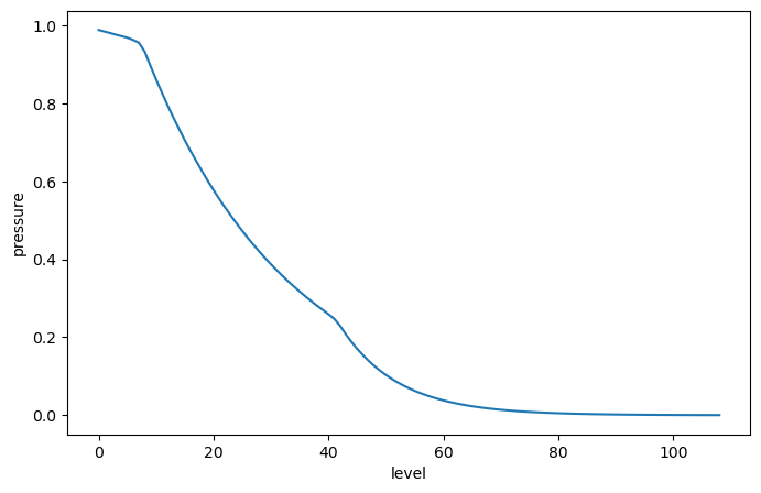
As a toy example, imagine we want to weight values in the upper ocean more than the lower ocean. We could imagine creating a weight array exponentially proportional to pressure as follows:
mean_pressure = argo.pressure.mean(dim='date')
p0 = 250 # dbat
weights = np.exp(-mean_pressure / p0)
weights.plot()
[<matplotlib.lines.Line2D at 0x7996fce5cbc0>]
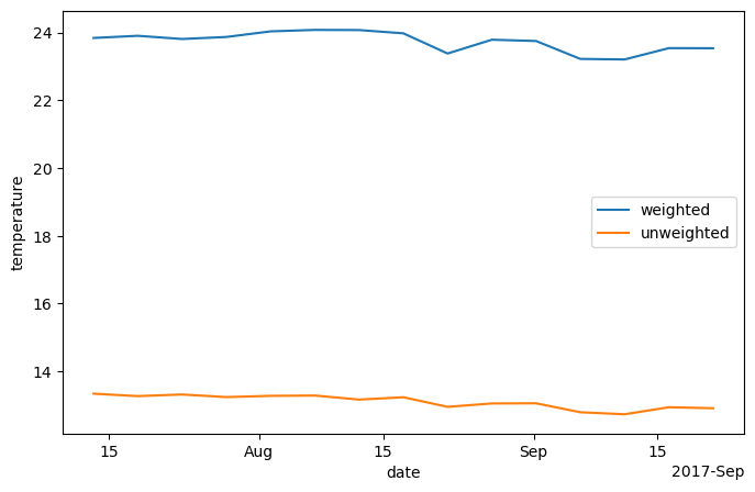
The weighted mean over the level dimensions is calculated as follows:
temp_weighted_mean = argo.temperature.weighted(weights).mean('level')
Comparing to the unweighted mean, we see the difference:
temp_weighted_mean.plot(label='weighted')
argo.temperature.mean(dim='level').plot(label='unweighted')
plt.legend()
<matplotlib.legend.Legend at 0x7997010306e0>
Loading Data from netCDF Files#
NetCDF (Network Common Data Format) is the most widely used format for distributing geoscience data. NetCDF is maintained by the Unidata organization.
Below we quote from the NetCDF website:
NetCDF (network Common Data Form) is a set of interfaces for array-oriented data access and a freely distributed collection of data access libraries for C, Fortran, C++, Java, and other languages. The netCDF libraries support a machine-independent format for representing scientific data. Together, the interfaces, libraries, and format support the creation, access, and sharing of scientific data.
NetCDF data is:
Self-Describing. A netCDF file includes information about the data it contains.
Portable. A netCDF file can be accessed by computers with different ways of storing integers, characters, and floating-point numbers.
Scalable. A small subset of a large dataset may be accessed efficiently.
Appendable. Data may be appended to a properly structured netCDF file without copying the dataset or redefining its structure.
Sharable. One writer and multiple readers may simultaneously access the same netCDF file.
Archivable. Access to all earlier forms of netCDF data will be supported by current and future versions of the software.
Xarray was designed to make reading netCDF files in python as easy, powerful, and flexible as possible. (See xarray netCDF docs for more details.)
Below we load some data from the LEAP catalog.
# https://catalog.leap.columbia.edu/feedstock/australian-gridded-climate-data-agcd
import xarray as xr
store = 'https://ncsa.osn.xsede.org/Pangeo/pangeo-forge/pangeo-forge/AGDC-feedstock/AGCD.zarr'
ds = xr.open_dataset(store, engine='zarr', chunks={})
ds
<xarray.Dataset> Size: 175GB
Dimensions: (lat: 691, lon: 886, time: 17897)
Coordinates:
* lat (lat) float32 3kB -44.5 -44.45 -44.4 ... -10.1 -10.05 -10.0
* lon (lon) float32 4kB 112.0 112.1 112.1 112.2 ... 156.1 156.2 156.2
* time (time) datetime64[ns] 143kB 1971-01-01T09:00:00 ... 2019-12-3...
Data variables:
precip (time, lat, lon) float32 44GB dask.array<chunksize=(40, 691, 886), meta=np.ndarray>
tmax (time, lat, lon) float32 44GB dask.array<chunksize=(40, 691, 886), meta=np.ndarray>
tmin (time, lat, lon) float32 44GB dask.array<chunksize=(40, 691, 886), meta=np.ndarray>
vapourpres (time, lat, lon) float32 44GB dask.array<chunksize=(40, 691, 886), meta=np.ndarray>
Attributes: (12/36)
Conventions: CF-1.6, ACDD-1.3
acknowledgment: The Australian Government, Bureau of Meteorolo...
agcd_version: AGCD (AWAP) v1.0.0 Snapshot (1900-01-01 to 202...
analysis_components: 0900: the gridded vapour pressure value at 9am...
attribution: Data should be cited as : Australian Bureau of...
cdm_data_type: Grid
... ...
summary: The partial pressure of water vapour in air (v...
time_coverage_end: 1971-12-31T00:00:00
time_coverage_start: 1971-01-01T15:00:00
title: Interpolated Vapour Pressure
url: http://www.bom.gov.au/climate/
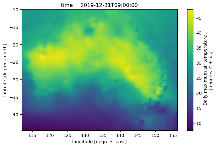
uuid: e684e0a6-73c7-4522-ab78-a8285ca34b4bds.tmax.isel(time=-1).plot()
<matplotlib.collections.QuadMesh at 0x7996daa828d0>
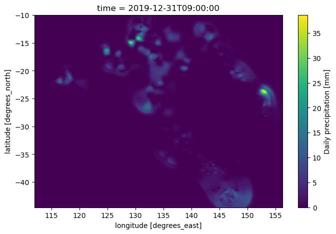
ds.precip.isel(time=-1).plot()
<matplotlib.collections.QuadMesh at 0x7996dab2b440>
# https://catalog.leap.columbia.edu/feedstock/aws-noaa-optimum-interpolated-sst
import xarray as xr
store = 'https://ncsa.osn.xsede.org/Pangeo/pangeo-forge/noaa_oisst/v2.1-avhrr.zarr'
ds = xr.open_dataset(store, engine='zarr', chunks={})
ds
<xarray.Dataset> Size: 241GB
Dimensions: (time: 14532, zlev: 1, lat: 720, lon: 1440)
Coordinates:
* lat (lat) float32 3kB -89.88 -89.62 -89.38 -89.12 ... 89.38 89.62 89.88
* lon (lon) float32 6kB 0.125 0.375 0.625 0.875 ... 359.4 359.6 359.9
* time (time) datetime64[ns] 116kB 1981-09-01T12:00:00 ... 2021-06-14T1...
* zlev (zlev) float32 4B 0.0
Data variables:
anom (time, zlev, lat, lon) float32 60GB dask.array<chunksize=(20, 1, 720, 1440), meta=np.ndarray>
err (time, zlev, lat, lon) float32 60GB dask.array<chunksize=(20, 1, 720, 1440), meta=np.ndarray>
ice (time, zlev, lat, lon) float32 60GB dask.array<chunksize=(20, 1, 720, 1440), meta=np.ndarray>
sst (time, zlev, lat, lon) float32 60GB dask.array<chunksize=(20, 1, 720, 1440), meta=np.ndarray>
Attributes: (12/37)
Conventions: CF-1.6, ACDD-1.3
cdm_data_type: Grid
comment: Data was converted from NetCDF-3 to NetCDF-4 ...
creator_email: oisst-help@noaa.gov
creator_url: https://www.ncei.noaa.gov/
date_created: 2020-05-08T19:05:13Z
... ...
source: ICOADS, NCEP_GTS, GSFC_ICE, NCEP_ICE, Pathfin...
standard_name_vocabulary: CF Standard Name Table (v40, 25 January 2017)
summary: NOAAs 1/4-degree Daily Optimum Interpolation ...
time_coverage_end: 1981-09-01T23:59:59Z
time_coverage_start: 1981-09-01T00:00:00Z
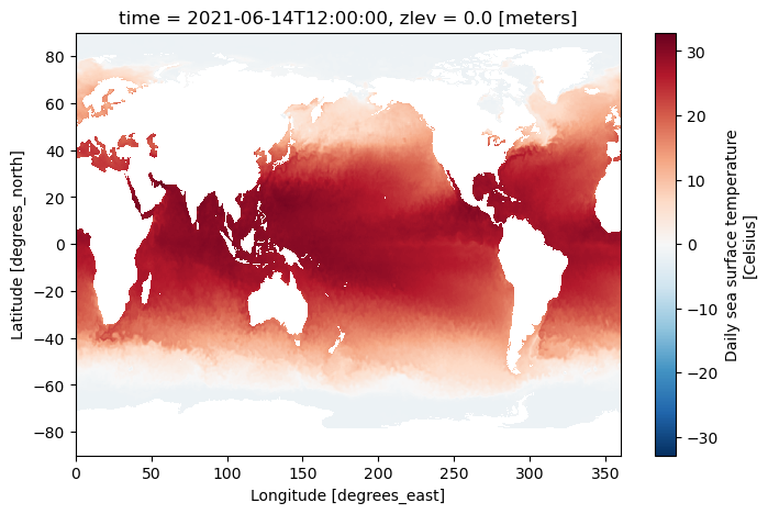
title: NOAA/NCEI 1/4 Degree Daily Optimum Interpolat...ds.sst.isel(time=-1, zlev=0).plot()
<matplotlib.collections.QuadMesh at 0x7996da211d30>
ds.time
<xarray.DataArray 'time' (time: 14532)> Size: 116kB
array(['1981-09-01T12:00:00.000000000', '1981-09-02T12:00:00.000000000',
'1981-09-03T12:00:00.000000000', ..., '2021-06-12T12:00:00.000000000',
'2021-06-13T12:00:00.000000000', '2021-06-14T12:00:00.000000000'],
shape=(14532,), dtype='datetime64[ns]')
Coordinates:
* time (time) datetime64[ns] 116kB 1981-09-01T12:00:00 ... 2021-06-14T1...
Attributes:
long_name: Center time of the dayXarray Tutorials:#
You can find a nice tutorial to fundamentals of Xarray on youtube here.
If you prefer reading there is a Xarray in 45 mins
And much much more: https://tutorial.xarray.dev/intro.html and https://www.youtube.com/playlist?list=PLNemzZpJM7lUu_iGP_lA2m7SeSUwKSIvR