Numpy and Matplotlib#
This lecture will introduce NumPy and Matplotlib. These are two of the most fundamental parts of the scientific python “ecosystem”. Most everything else is built on top of them.
Numpy: The fundamental package for scientific computing with Python
Website: https://numpy.org/
GitHub: numpy/numpy
Matlotlib: Matplotlib is a comprehensive library for creating static, animated, and interactive visualizations in Python.
Website: https://matplotlib.org/
GitHub: matplotlib/matplotlib
Importing and Examining a New Package#
This will be our first experience with importing a package which is not part of the Python standard library.
import numpy as np
What did we just do? We imported a package. This brings new variables (mostly functions) into our interpreter. We access them as follows.
# find out what is in our namespace
dir()
['In',
 'Out',
 '_',
 '__',
 '___',
 '__builtin__',
 '__builtins__',
 '__doc__',
 '__loader__',
 '__name__',
 '__package__',
 '__spec__',
 '_dh',
 '_i',
 '_i1',
 '_i2',
 '_ih',
 '_ii',
 '_iii',
 '_oh',
 'exit',
 'get_ipython',
 'np',
 'open',
 'quit']
# find out what's in numpy
dir(np)
['False_',
 'ScalarType',
 'True_',
 '_CopyMode',
 '_NoValue',
 '__NUMPY_SETUP__',
 '__all__',
 '__array_api_version__',
 '__array_namespace_info__',
 '__builtins__',
 '__cached__',
 '__config__',
 '__dir__',
 '__doc__',
 '__expired_attributes__',
 '__file__',
 '__former_attrs__',
 '__future_scalars__',
 '__getattr__',
 '__loader__',
 '__name__',
 '__numpy_submodules__',
 '__package__',
 '__path__',
 '__spec__',
 '__version__',
 '_array_api_info',
 '_core',
 '_distributor_init',
 '_expired_attrs_2_0',
 '_globals',
 '_int_extended_msg',
 '_mat',
 '_msg',
 '_pyinstaller_hooks_dir',
 '_pytesttester',
 '_specific_msg',
 '_type_info',
 '_typing',
 '_utils',
 'abs',
 'absolute',
 'acos',
 'acosh',
 'add',
 'all',
 'allclose',
 'amax',
 'amin',
 'angle',
 'any',
 'append',
 'apply_along_axis',
 'apply_over_axes',
 'arange',
 'arccos',
 'arccosh',
 'arcsin',
 'arcsinh',
 'arctan',
 'arctan2',
 'arctanh',
 'argmax',
 'argmin',
 'argpartition',
 'argsort',
 'argwhere',
 'around',
 'array',
 'array2string',
 'array_equal',
 'array_equiv',
 'array_repr',
 'array_split',
 'array_str',
 'asanyarray',
 'asarray',
 'asarray_chkfinite',
 'ascontiguousarray',
 'asfortranarray',
 'asin',
 'asinh',
 'asmatrix',
 'astype',
 'atan',
 'atan2',
 'atanh',
 'atleast_1d',
 'atleast_2d',
 'atleast_3d',
 'average',
 'bartlett',
 'base_repr',
 'binary_repr',
 'bincount',
 'bitwise_and',
 'bitwise_count',
 'bitwise_invert',
 'bitwise_left_shift',
 'bitwise_not',
 'bitwise_or',
 'bitwise_right_shift',
 'bitwise_xor',
 'blackman',
 'block',
 'bmat',
 'bool',
 'bool_',
 'broadcast',
 'broadcast_arrays',
 'broadcast_shapes',
 'broadcast_to',
 'busday_count',
 'busday_offset',
 'busdaycalendar',
 'byte',
 'bytes_',
 'c_',
 'can_cast',
 'cbrt',
 'cdouble',
 'ceil',
 'char',
 'character',
 'choose',
 'clip',
 'clongdouble',
 'column_stack',
 'common_type',
 'complex128',
 'complex256',
 'complex64',
 'complexfloating',
 'compress',
 'concat',
 'concatenate',
 'conj',
 'conjugate',
 'convolve',
 'copy',
 'copysign',
 'copyto',
 'core',
 'corrcoef',
 'correlate',
 'cos',
 'cosh',
 'count_nonzero',
 'cov',
 'cross',
 'csingle',
 'ctypeslib',
 'cumprod',
 'cumsum',
 'cumulative_prod',
 'cumulative_sum',
 'datetime64',
 'datetime_as_string',
 'datetime_data',
 'deg2rad',
 'degrees',
 'delete',
 'diag',
 'diag_indices',
 'diag_indices_from',
 'diagflat',
 'diagonal',
 'diff',
 'digitize',
 'divide',
 'divmod',
 'dot',
 'double',
 'dsplit',
 'dstack',
 'dtype',
 'dtypes',
 'e',
 'ediff1d',
 'einsum',
 'einsum_path',
 'emath',
 'empty',
 'empty_like',
 'equal',
 'errstate',
 'euler_gamma',
 'exceptions',
 'exp',
 'exp2',
 'expand_dims',
 'expm1',
 'extract',
 'eye',
 'f2py',
 'fabs',
 'fft',
 'fill_diagonal',
 'finfo',
 'fix',
 'flatiter',
 'flatnonzero',
 'flexible',
 'flip',
 'fliplr',
 'flipud',
 'float128',
 'float16',
 'float32',
 'float64',
 'float_power',
 'floating',
 'floor',
 'floor_divide',
 'fmax',
 'fmin',
 'fmod',
 'format_float_positional',
 'format_float_scientific',
 'frexp',
 'from_dlpack',
 'frombuffer',
 'fromfile',
 'fromfunction',
 'fromiter',
 'frompyfunc',
 'fromregex',
 'fromstring',
 'full',
 'full_like',
 'gcd',
 'generic',
 'genfromtxt',
 'geomspace',
 'get_include',
 'get_printoptions',
 'getbufsize',
 'geterr',
 'geterrcall',
 'gradient',
 'greater',
 'greater_equal',
 'half',
 'hamming',
 'hanning',
 'heaviside',
 'histogram',
 'histogram2d',
 'histogram_bin_edges',
 'histogramdd',
 'hsplit',
 'hstack',
 'hypot',
 'i0',
 'identity',
 'iinfo',
 'imag',
 'in1d',
 'index_exp',
 'indices',
 'inexact',
 'inf',
 'info',
 'inner',
 'insert',
 'int16',
 'int32',
 'int64',
 'int8',
 'int_',
 'intc',
 'integer',
 'interp',
 'intersect1d',
 'intp',
 'invert',
 'is_busday',
 'isclose',
 'iscomplex',
 'iscomplexobj',
 'isdtype',
 'isfinite',
 'isfortran',
 'isin',
 'isinf',
 'isnan',
 'isnat',
 'isneginf',
 'isposinf',
 'isreal',
 'isrealobj',
 'isscalar',
 'issubdtype',
 'iterable',
 'ix_',
 'kaiser',
 'kron',
 'lcm',
 'ldexp',
 'left_shift',
 'less',
 'less_equal',
 'lexsort',
 'lib',
 'linalg',
 'linspace',
 'little_endian',
 'load',
 'loadtxt',
 'log',
 'log10',
 'log1p',
 'log2',
 'logaddexp',
 'logaddexp2',
 'logical_and',
 'logical_not',
 'logical_or',
 'logical_xor',
 'logspace',
 'long',
 'longdouble',
 'longlong',
 'ma',
 'mask_indices',
 'matmul',
 'matrix',
 'matrix_transpose',
 'matvec',
 'max',
 'maximum',
 'may_share_memory',
 'mean',
 'median',
 'memmap',
 'meshgrid',
 'mgrid',
 'min',
 'min_scalar_type',
 'minimum',
 'mintypecode',
 'mod',
 'modf',
 'moveaxis',
 'multiply',
 'nan',
 'nan_to_num',
 'nanargmax',
 'nanargmin',
 'nancumprod',
 'nancumsum',
 'nanmax',
 'nanmean',
 'nanmedian',
 'nanmin',
 'nanpercentile',
 'nanprod',
 'nanquantile',
 'nanstd',
 'nansum',
 'nanvar',
 'ndarray',
 'ndenumerate',
 'ndim',
 'ndindex',
 'nditer',
 'negative',
 'nested_iters',
 'newaxis',
 'nextafter',
 'nonzero',
 'not_equal',
 'number',
 'object_',
 'ogrid',
 'ones',
 'ones_like',
 'outer',
 'packbits',
 'pad',
 'partition',
 'percentile',
 'permute_dims',
 'pi',
 'piecewise',
 'place',
 'poly',
 'poly1d',
 'polyadd',
 'polyder',
 'polydiv',
 'polyfit',
 'polyint',
 'polymul',
 'polynomial',
 'polysub',
 'polyval',
 'positive',
 'pow',
 'power',
 'printoptions',
 'prod',
 'promote_types',
 'ptp',
 'put',
 'put_along_axis',
 'putmask',
 'quantile',
 'r_',
 'rad2deg',
 'radians',
 'random',
 'ravel',
 'ravel_multi_index',
 'real',
 'real_if_close',
 'rec',
 'recarray',
 'reciprocal',
 'record',
 'remainder',
 'repeat',
 'require',
 'reshape',
 'resize',
 'result_type',
 'right_shift',
 'rint',
 'roll',
 'rollaxis',
 'roots',
 'rot90',
 'round',
 'row_stack',
 's_',
 'save',
 'savetxt',
 'savez',
 'savez_compressed',
 'sctypeDict',
 'searchsorted',
 'select',
 'set_printoptions',
 'setbufsize',
 'setdiff1d',
 'seterr',
 'seterrcall',
 'setxor1d',
 'shape',
 'shares_memory',
 'short',
 'show_config',
 'show_runtime',
 'sign',
 'signbit',
 'signedinteger',
 'sin',
 'sinc',
 'single',
 'sinh',
 'size',
 'sort',
 'sort_complex',
 'spacing',
 'split',
 'sqrt',
 'square',
 'squeeze',
 'stack',
 'std',
 'str_',
 'strings',
 'subtract',
 'sum',
 'swapaxes',
 'take',
 'take_along_axis',
 'tan',
 'tanh',
 'tensordot',
 'test',
 'testing',
 'tile',
 'timedelta64',
 'trace',
 'transpose',
 'trapezoid',
 'trapz',
 'tri',
 'tril',
 'tril_indices',
 'tril_indices_from',
 'trim_zeros',
 'triu',
 'triu_indices',
 'triu_indices_from',
 'true_divide',
 'trunc',
 'typecodes',
 'typename',
 'typing',
 'ubyte',
 'ufunc',
 'uint',
 'uint16',
 'uint32',
 'uint64',
 'uint8',
 'uintc',
 'uintp',
 'ulong',
 'ulonglong',
 'union1d',
 'unique',
 'unique_all',
 'unique_counts',
 'unique_inverse',
 'unique_values',
 'unpackbits',
 'unravel_index',
 'unsignedinteger',
 'unstack',
 'unwrap',
 'ushort',
 'vander',
 'var',
 'vdot',
 'vecdot',
 'vecmat',
 'vectorize',
 'void',
 'vsplit',
 'vstack',
 'where',
 'zeros',
 'zeros_like']
# find out what version we have
np.__version__
'2.2.6'
There is no way we could explicitly teach each of these functions. The numpy documentation is crucial!
NDArrays#
The core class is the numpy ndarray (n-dimensional array).
The main difference between a numpy array an a more general data container such as list are the following:
Numpy arrays can have N dimensions (while lists, tuples, etc. only have 1)
Numpy arrays hold values of the same datatype (e.g.
int,float), whilelistscan contain anything.Numpy optimizes numerical operations on arrays. Numpy is fast!
# create an array from a list
a = np.array([9,0,2,1,0])
# find out the datatype
a.dtype
dtype('int64')
# find out the shape
a.shape
(5,)
# what is the shape
type(a.shape)
tuple
# another array with a different datatype and shape
b = np.array([[5,3,1,9],[9,2,3,0]], dtype=np.float64)

# check dtype and shape
b.dtype, b.shape
(dtype('float64'), (2, 4))
Note
The fastest varying dimension is the last dimension! The outer level of the hierarchy is the first dimension. (This is called “c-style” indexing)
Array Creation#
There are lots of ways to create arrays.
# create some uniform arrays
c = np.zeros((9,9))
d = np.ones((3,6,3), dtype=np.complex128)
e = np.full((3,3), np.pi)
e = np.ones_like(c)
f = np.zeros_like(d)
arange works very similar to range, but it populates the array “eagerly” (i.e. immediately), rather than generating the values upon iteration.
np.arange(10)
array([0, 1, 2, 3, 4, 5, 6, 7, 8, 9])
arange is left inclusive, right exclusive, just like range, but also works with floating-point numbers.
np.arange(2,4,0.25)
array([2. , 2.25, 2.5 , 2.75, 3. , 3.25, 3.5 , 3.75])
A frequent need is to generate an array of N numbers, evenly spaced between two values. That is what linspace is for.
np.linspace(2,4,20)
array([2.        , 2.10526316, 2.21052632, 2.31578947, 2.42105263,
       2.52631579, 2.63157895, 2.73684211, 2.84210526, 2.94736842,
       3.05263158, 3.15789474, 3.26315789, 3.36842105, 3.47368421,
       3.57894737, 3.68421053, 3.78947368, 3.89473684, 4.        ])
# log spaced
np.logspace(1,2,10)
array([ 10.        ,  12.91549665,  16.68100537,  21.5443469 ,
        27.82559402,  35.93813664,  46.41588834,  59.94842503,
        77.42636827, 100.        ])
Numpy also has some utilities for helping us generate multi-dimensional arrays.
meshgrid creates 2D arrays out of a combination of 1D arrays. Meshgrid essentially tiles 1D arrays to a shape that is combined shape of the input arrays.
x = np.linspace(-2*np.pi, 2*np.pi, 100)
y = np.linspace(-np.pi, np.pi, 50)
xx, yy = np.meshgrid(x, y)
print(x.shape, y.shape)
print(xx.shape, yy.shape)
(100,) (50,)
(50, 100) (50, 100)
Indexing#
Basic indexing is similar to lists
# get some individual elements of y
y[10], y[1:5], y[-5]
(np.float64(-1.8593099378388573),
 array([-3.01336438, -2.88513611, -2.75690784, -2.62867957]),
 np.float64(2.628679567289418))
# get some individual elements of xx
xx[0,0], xx[-1,-1], xx[3,-5]
(np.float64(-6.283185307179586),
 np.float64(6.283185307179586),
 np.float64(5.775453161144872))
# get some whole rows and columns
xx[0].shape, xx[:,-1].shape
((100,), (50,))
# get some ranges
xx[3:10,30:40].shape
(7, 10)
There are many advanced ways to index arrays. You can read about them in the manual. Here is one example.
# use a boolean array as an index
idx = xx<0
yy[idx].shape
(2500,)
# the array got flattened
xx.ravel().shape
(5000,)
Visualizing Arrays with Matplotlib#
It can be hard to work with big arrays without actually seeing anything with our eyes! We will now bring in Matplotib to start visualizating these arrays.
from matplotlib import pyplot as plt
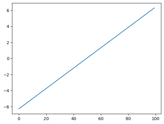
For plotting a 1D array as a line, we use the plot command.
plt.plot(x)
[<matplotlib.lines.Line2D at 0x7cd8af7e0cb0>]
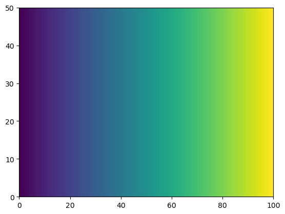
There are many ways to visualize 2D data.
He we use pcolormesh.
plt.pcolormesh(xx)
<matplotlib.collections.QuadMesh at 0x7cd8af7e08f0>
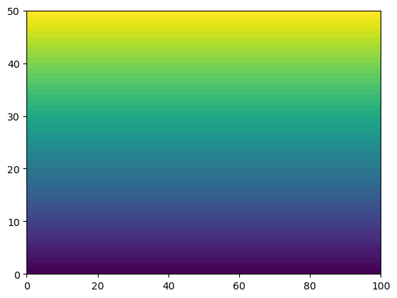
plt.pcolormesh(yy)
<matplotlib.collections.QuadMesh at 0x7cd8af64dc70>
Array Operations#
There are a huge number of operations available on arrays. All the familiar arithemtic operators are applied on an element-by-element basis.
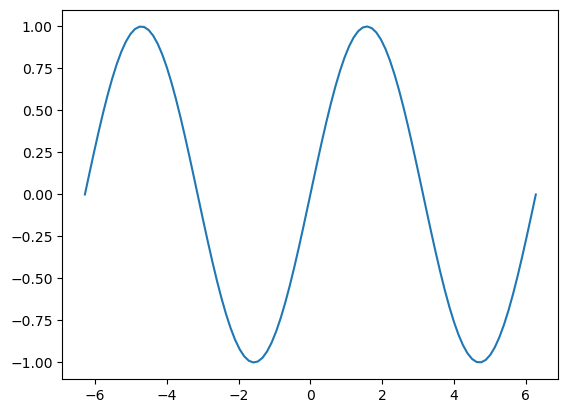
Basic Math#
# y = f(x)
f = np.sin(x)
plt.plot(x, f)
[<matplotlib.lines.Line2D at 0x7cd8af6ecfb0>]
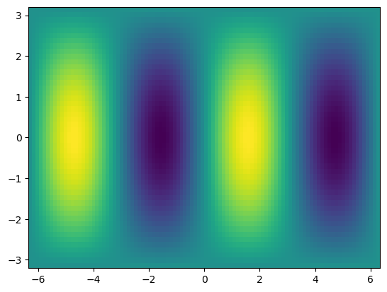
# z = f(x,y), where z is a 2D surface defined a grid in the x and y directions.
# Here we use the 2D version of x and y,
# so that we know the values of x and y at all grid points.
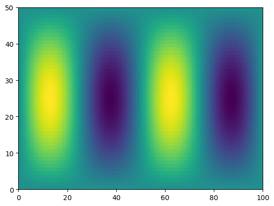
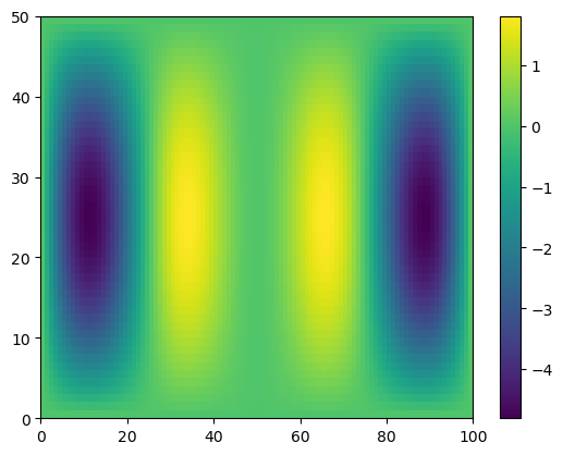
f = np.sin(xx) * np.cos(0.5*yy)
plt.pcolormesh(xx,yy,f)
<matplotlib.collections.QuadMesh at 0x7cd8af7e0830>
Manipulating array dimensions#
Swapping the dimension order is accomplished by calling transpose.
f_transposed = f.transpose()
plt.pcolormesh(f_transposed)
<matplotlib.collections.QuadMesh at 0x7cd8af630410>
We can also manually change the shape of an array…as long as the new shape has the same number of elements.
g = np.reshape(f, (8,9))
----------------------------------------------------------------
ValueError                     Traceback (most recent call last)
Cell In[31], line 1
----> 1 g = np.reshape(f, (8,9))

File /srv/conda/envs/notebook/lib/python3.12/site-packages/numpy/_core/fromnumeric.py:324, in reshape(a, shape, order, newshape, copy)
    322 if copy is not None:
    323     return _wrapfunc(a, 'reshape', shape, order=order, copy=copy)
--> 324 return _wrapfunc(a, 'reshape', shape, order=order)

File /srv/conda/envs/notebook/lib/python3.12/site-packages/numpy/_core/fromnumeric.py:57, in _wrapfunc(obj, method, *args, **kwds)
     54     return _wrapit(obj, method, *args, **kwds)
     56 try:
---> 57     return bound(*args, **kwds)
     58 except TypeError:
     59     # A TypeError occurs if the object does have such a method in its
     60     # class, but its signature is not identical to that of NumPy's. This
   (...)
     64     # Call _wrapit from within the except clause to ensure a potential
     65     # exception has a traceback chain.
     66     return _wrapit(obj, method, *args, **kwds)

ValueError: cannot reshape array of size 5000 into shape (8,9)
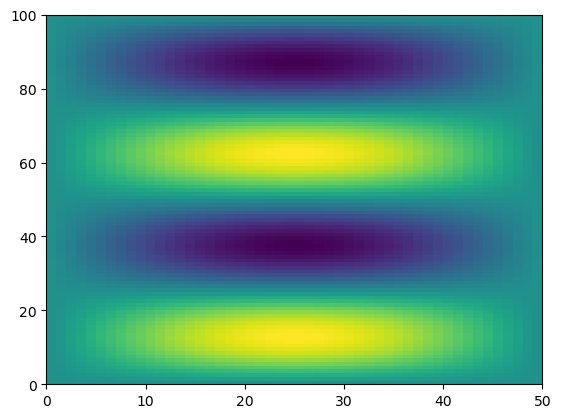
However, be careful with reshapeing data! You can accidentally lose the structure of the data.
g = np.reshape(f, (200,25))
plt.pcolormesh(g)
<matplotlib.collections.QuadMesh at 0x7cd8a72f8c80>
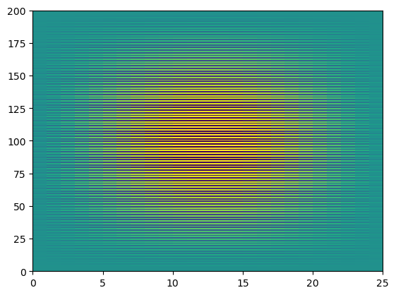
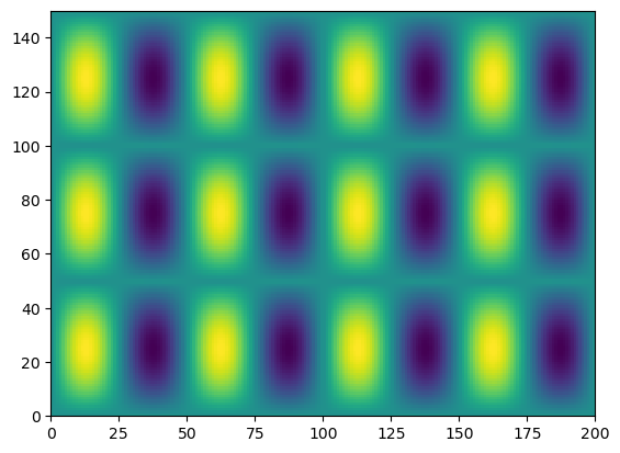
We can also “tile” an array to repeat it many times.
f_tiled = np.tile(f,(3, 2))
plt.pcolormesh(f_tiled)
<matplotlib.collections.QuadMesh at 0x7cd8a732b440>
Another common need is to add an extra dimension to an array.
This can be accomplished via indexing with None.
x.shape
(100,)
x[None, :].shape
(1, 100)
x[None, :, None, None].shape
(1, 100, 1, 1)
Broadcasting#
Not all the arrays we want to work with will have the same size.
One approach would be to manually “expand” our arrays to all be the same size, e.g. using tile.
Broadcasting is a more efficient way to multiply arrays of different sizes
Numpy has specific rules for how broadcasting works.
These can be confusing but are worth learning if you plan to work with Numpy data a lot.
The core concept of broadcasting is telling Numpy which dimensions are supposed to line up with each other.
from IPython.display import Image
Image(url='http://scipy-lectures.github.io/_images/numpy_broadcasting.png',
     width=720)
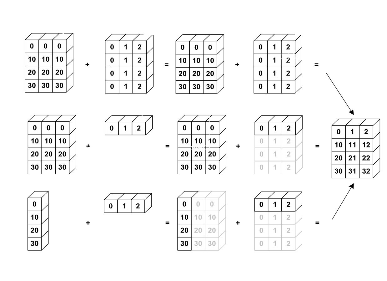
General Broadcasting Rules: When performing operations on two arrays, NumPy compares their shapes element-wise starting from the trailing dimensions (right to left). It follows these rules:
If the dimensions are equal, they’re compatible.
If one of the dimensions is 1, it’s “stretched” to match the other.
If the dimensions are unequal and neither is 1, the arrays are not broadcastable.
print(f.shape, x.shape)
g = f * x
print(g.shape)
(50, 100) (100,)
(50, 100)
plt.pcolormesh(f)
<matplotlib.collections.QuadMesh at 0x7cd8a736cdd0>
plt.pcolormesh(g)
<matplotlib.collections.QuadMesh at 0x7cd8af835850>
However, if the last two dimensions are not the same, Numpy cannot just automatically figure it out.
# multiply f by y
print(f.shape, y.shape)
h = f * y
(50, 100) (50,)
----------------------------------------------------------------
ValueError                     Traceback (most recent call last)
Cell In[41], line 3
      1 # multiply f by y
      2 print(f.shape, y.shape)
----> 3 h = f * y

ValueError: operands could not be broadcast together with shapes (50,100) (50,)
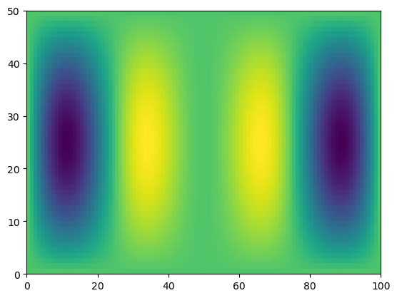
We can help numpy by adding an extra dimension to y at the end.
Then the length-50 dimensions will line up.
print(f.shape, y[:, None].shape)
h = f * y[:, None]
print(h.shape)
(50, 100) (50, 1)
(50, 100)
plt.pcolormesh(h)
<matplotlib.collections.QuadMesh at 0x7cd8a7227680>
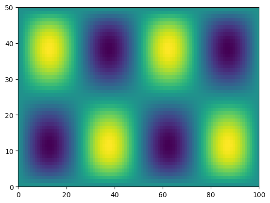
Exercise#
Can you create and plot the f = np.sin(xx) * np.cos(0.5*yy) from before, but using the 1-D x and y and broadcasting?
x.shape
(100,)
x[None,:].shape
(1, 100)
y.shape
(50,)
y[:,None].shape
(50, 1)
f = np.sin(x[None,:]) * np.cos(0.5*y[:,None])
plt.pcolormesh(f)
<matplotlib.collections.QuadMesh at 0x7cd8a737bad0>
Reduction Operations#
In scientific data analysis, we usually start with a lot of data and want to reduce it down in order to make plots of summary tables. Operations that reduce the size of numpy arrays are called “reductions”. There are many different reduction operations. Here we will look at some of the most common ones.
# sum
g.sum()
np.float64(-3083.038387807155)
# mean
g.mean()
np.float64(-0.616607677561431)
# standard deviation
g.std()
np.float64(1.6402280119141424)
A key property of numpy reductions is the ability to operate on just one axis.
plt.pcolormesh(g)
plt.colorbar()
<matplotlib.colorbar.Colorbar at 0x7cd8a7225e50>
temp2 = g.shape
temp2
(50, 100)
temp2[1]
100
temp = np.ones((100,50,25))
# apply on just one axis
g_ymean = g.mean(axis=0)
g_xmean = g.mean(axis=1)
temp3 = temp.shape
temp3
(100, 50, 25)
temp3[1]
50
temp.mean(axis=(0,1,2))
np.float64(1.0)
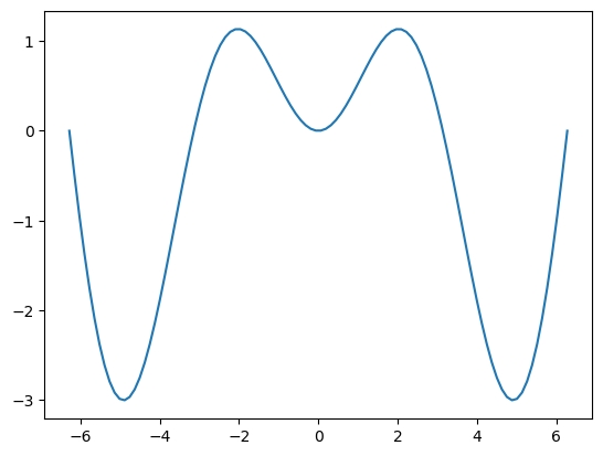
plt.plot(x, g_ymean)
[<matplotlib.lines.Line2D at 0x7cd8a6a9b740>]
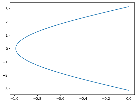
plt.plot(g_xmean, y)
[<matplotlib.lines.Line2D at 0x7cd8a693ee40>]
g
array([[-9.42326863e-32, -4.77205105e-17, -9.27211559e-17, ...,
        -9.27211559e-17, -4.77205105e-17, -9.42326863e-32],
       [-9.86000036e-17, -4.99321700e-02, -9.70184196e-02, ...,
        -9.70184196e-02, -4.99321700e-02, -9.86000036e-17],
       [-1.96794839e-16, -9.96591580e-02, -1.93638170e-01, ...,
        -1.93638170e-01, -9.96591580e-02, -1.96794839e-16],
       ...,
       [-1.96794839e-16, -9.96591580e-02, -1.93638170e-01, ...,
        -1.93638170e-01, -9.96591580e-02, -1.96794839e-16],
       [-9.86000036e-17, -4.99321700e-02, -9.70184196e-02, ...,
        -9.70184196e-02, -4.99321700e-02, -9.86000036e-17],
       [-9.42326863e-32, -4.77205105e-17, -9.27211559e-17, ...,
        -9.27211559e-17, -4.77205105e-17, -9.42326863e-32]],
      shape=(50, 100))
g.shape
(50, 100)
Data Files#
It can be useful to save numpy data into files.
np.save('g.npy', g)
Warning
Numpy .npy files are a convenient way to store temporary data, but they are not considered a robust archival format.
Later we will learn about NetCDF, the recommended way to store earth and environmental data.
g_loaded = np.load('g.npy')
g_loaded
array([[-9.42326863e-32, -4.77205105e-17, -9.27211559e-17, ...,
        -9.27211559e-17, -4.77205105e-17, -9.42326863e-32],
       [-9.86000036e-17, -4.99321700e-02, -9.70184196e-02, ...,
        -9.70184196e-02, -4.99321700e-02, -9.86000036e-17],
       [-1.96794839e-16, -9.96591580e-02, -1.93638170e-01, ...,
        -1.93638170e-01, -9.96591580e-02, -1.96794839e-16],
       ...,
       [-1.96794839e-16, -9.96591580e-02, -1.93638170e-01, ...,
        -1.93638170e-01, -9.96591580e-02, -1.96794839e-16],
       [-9.86000036e-17, -4.99321700e-02, -9.70184196e-02, ...,
        -9.70184196e-02, -4.99321700e-02, -9.86000036e-17],
       [-9.42326863e-32, -4.77205105e-17, -9.27211559e-17, ...,
        -9.27211559e-17, -4.77205105e-17, -9.42326863e-32]],
      shape=(50, 100))
np.testing.assert_equal(g, g_loaded*0.5)
----------------------------------------------------------------
AssertionError                 Traceback (most recent call last)
Cell In[70], line 1
----> 1 np.testing.assert_equal(g, g_loaded*0.5)

    [... skipping hidden 3 frame]

File /srv/conda/envs/notebook/lib/python3.12/site-packages/numpy/testing/_private/utils.py:921, in assert_array_compare(comparison, x, y, err_msg, verbose, header, precision, equal_nan, equal_inf, strict, names)
    916         err_msg += '\n' + '\n'.join(remarks)
    917         msg = build_err_msg([ox, oy], err_msg,
    918                             verbose=verbose, header=header,
    919                             names=names,
    920                             precision=precision)
--> 921         raise AssertionError(msg)
    922 except ValueError:
    923     import traceback

AssertionError:
Arrays are not equal

Mismatched elements: 5000 / 5000 (100%)
Max absolute difference among violations: 2.40510295
Max relative difference among violations: 1.
 ACTUAL: array([[-9.423269e-32, -4.772051e-17, -9.272116e-17, ..., -9.272116e-17,
        -4.772051e-17, -9.423269e-32],
       [-9.860000e-17, -4.993217e-02, -9.701842e-02, ..., -9.701842e-02,...
 DESIRED: array([[-4.711634e-32, -2.386026e-17, -4.636058e-17, ..., -4.636058e-17,
        -2.386026e-17, -4.711634e-32],
       [-4.930000e-17, -2.496608e-02, -4.850921e-02, ..., -4.850921e-02,...
np.testing.assert_equal(g, g_loaded)