
Formats and metadata#
This page is a short tour of the kinds of data you’ll meet in climate and environmental science, how they’re stored, and how to think about metadata and sharing.
What is data?#
For our purposes, scientific data is organized information stored on disk. What you can do with a dataset depends on its format — how the values are arranged in the file and what conventions are used to describe them. The format determines which Python tools can read it, what structure you’ll get back, and whether the metadata travels along with the values.
Most of this lecture is about recognizing the main formats you’ll meet in this course, and how to think about the metadata and licensing that come with them.
Common data formats#
Single values only get you so far. To represent scientific data, you need ways of organizing many values together. In this course you’ll mostly encounter three families.
Tabular data#
Rows and columns, like a spreadsheet. Each row is an observation, each column a variable. For example:
Name |
Mass |
Diameter |
|---|---|---|
Mercury |
0.330 × 10²⁴ kg |
4879 km |
Venus |
4.87 × 10²⁴ kg |
12104 km |
Earth |
5.97 × 10²⁴ kg |
12756 km |
(via NASA’s Planetary Fact Sheet)
Common storage:
CSV (comma-separated values) — human-readable plain text, universally supported, but no built-in types or metadata. Most common.
Parquet — columnar binary format, much more efficient for large tables, but not human-readable.
In Python, tabular data lives in pandas (covered later in this course).
Gridded (array) data#
Numerical data on N-dimensional regular grids — temperature at every (latitude, longitude, time), for example.
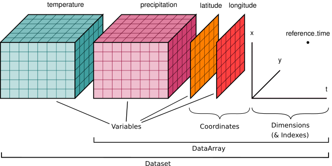
(via xarray docs)
Common storage:
NetCDF — long-time standard in earth sciences. Self-describing: variables, dimensions, units, and other metadata are embedded in the file.
Zarr — newer, cloud-native equivalent. Stores arrays as collections of small “chunks,” much better suited to streaming over the network.
HDF5 — generic hierarchical container that NetCDF is built on top of.
In Python, gridded data lives in xarray (covered later in this course).
Raster (image) data#
A specific kind of gridded data: 2D pixel arrays with a geographic coordinate reference system. Used for satellite imagery, digital elevation models, etc.

(image credit: Environmental Systems Research Institute, Inc.)
Common storage:
GeoTIFF — the most common format. Includes the coordinate reference system in the file’s metadata so each pixel maps to a location on Earth.
Cloud-optimized GeoTIFF (CoG) — newer variant designed for streaming subsets over HTTP.
In Python, raster data is commonly read with rasterio (or rioxarray for xarray-style access).
Vector data#
Discrete geometric features on the Earth’s surface — points (cities, sensors), lines (rivers, roads), or polygons (countries, watersheds).
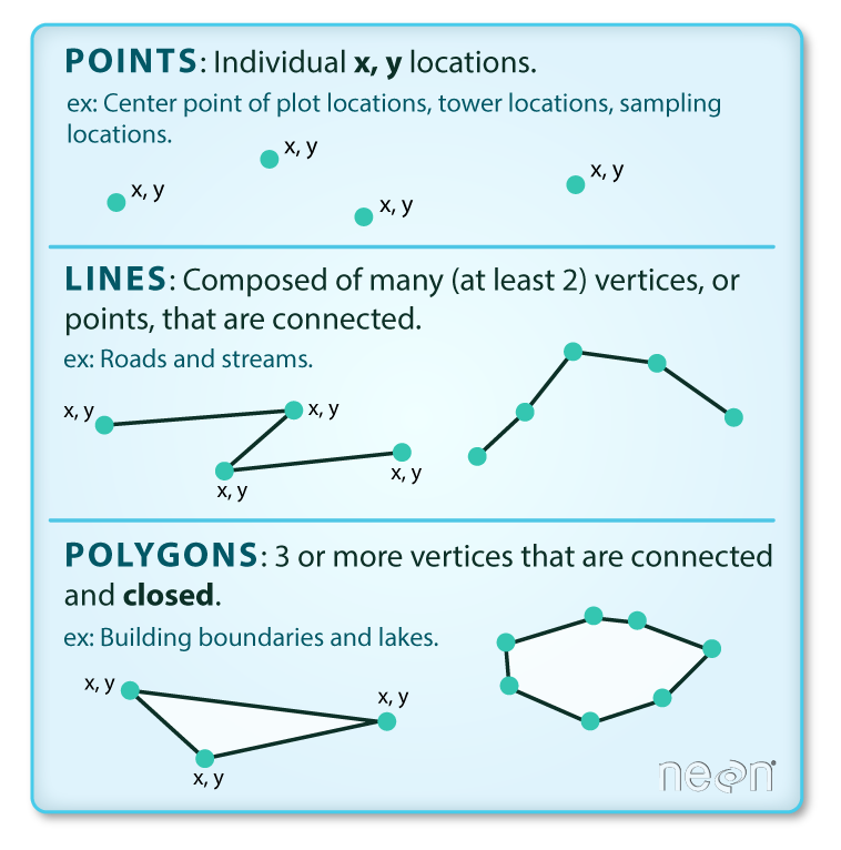
(image credit: National Ecological Observatory Network (NEON), via Data Carpentry)
Common storage:
ESRI Shapefile — long-standing, widely supported (despite its flaws).
GeoJSON — JSON-based, human-readable.
GeoPackage / FlatGeoBuf — modern alternatives.
In Python, vector data is read with Fiona or GeoPandas. We won’t use vector data much in this course, but you’ll likely meet it later.
Reference: Other data shapes you may run into — graph data (nodes and edges, handled in Python with NetworkX), unstructured / nested data (commonly stored as JSON), or relational databases for sets of related tables. They’re not central to this course, but it’s worth knowing they exist.
Metadata#
Metadata is “data about the data”: who created it, when, with what instrument, what units, what coordinate system, what license. Without metadata, raw numbers are nearly useless.
In earth science, common metadata conventions for NetCDF/Zarr data include:
CF Conventions — Climate and Forecast standard names, units, coordinate system descriptors.
Attribute Convention for Data Discovery (ACDD) — discovery-level fields like title, summary, geographic extent.
For CSV or other formats without embedded metadata, a separate README.txt or similar is the standard.
FAIR data#
Modern scientific practice is converging on a shared standard for what makes data shareable and useful. The acronym is FAIR:
Findable — has a persistent identifier (like a DOI) and rich, indexed metadata.
Accessible — retrievable via a standard, open protocol (HTTP, OPeNDAP, etc.).
Interoperable — uses formal, shared vocabularies (e.g., CF Conventions).
Reusable — released with a clear license and provenance information.
Reference: The full FAIR principles go into more detail, but the four words above cover the core ideas.
Persistent identifiers and DOIs#
The most important FAIR practice for getting data is the Digital Object Identifier (DOI) — a permanent, citeable URL for a dataset (or paper, or piece of software). A DOI looks like:
10.5281/zenodo.5739406
and is resolved by prepending https://doi.org/:
https://doi.org/10.5281/zenodo.5739406
Publishers and data repositories commit to keeping DOIs working “forever.” If your code references data by DOI (rather than an arbitrary URL), it stays reproducible even if the data is later moved or reorganized.