Pandas: Groupby

Often we don’t want a single summary for the whole dataset — we want one value per group: the average temperature in each month, the strongest earthquake in each country, the total rainfall in each year. groupby is the tool for exactly this, and it’s one of the most useful things pandas does.

The pattern it follows is called split–apply–combine: split the rows into groups, apply a calculation to each group, then combine the results back together. We’ll build that intuition on two datasets — first grouping earthquakes by country, then grouping a weather station’s daily record by time to build climatologies and anomalies. Along the way we’ll meet groupby’s close relatives resample (grouping by time interval) and rolling (moving-window calculations).

These notes draw on the pandas groupby documentation; the split-apply-combine framing comes from a paper by Hadley Wickham.

Working through this notebook

This page is a Jupyter notebook. Download it using the ⬇ button in the top-right (or copy-paste the cells into a fresh notebook), open it in your environment (JupyterLab on LEAP or Colab), and step through the cells. When you reach a Try it admonition, experiment in your own cells before moving on.

In-class assignment — 10 points

The “Try it” exercises in this notebook are part of your in-class assignment for this section. Complete them in your own copy of the notebook, push it to your week folder, and post the notebook link on the matching Courseworks assignment. (One 10-point assignment covers all the lecture notebooks in this section.)

import numpy as np
from matplotlib import pyplot as plt
plt.rcParams['figure.figsize'] = (12,7)
%matplotlib inline
import pandas as pd

First we read the earthquake data from the previous assignment. Two extra steps set up the rest of the lesson: we derive a country column from the free-text place field, and we split the catalog by magnitude into the larger events (df, magnitude > 4) and the smaller ones (df_small, magnitude < 4), so we can compare the two groups later.

df = pd.read_csv('https://raw.githubusercontent.com/earth-DS-ML/summer_2026/refs/heads/main/lectures_DS/data/usgs_earthquakes_2025.csv', parse_dates=['time'], index_col='id')
df['country'] = df.place.str.split(', ').str[-1]
df_small = df[df.mag<4]
df = df[df.mag>4]
df.head()

	time	latitude	longitude	depth	mag	magType	nst	gap	dmin	rms	...	place	type	horizontalError	depthError	magError	magNst	status	locationSource	magSource	country
id
us6000qkt1	2025-06-17 12:00:22.773000+00:00	-23.1645	-175.3549	10.000	4.9	mb	22.0	166.0	6.481	0.49	...	206 km SSW of ‘Ohonua, Tonga	earthquake	15.85	1.938	0.093	36.0	reviewed	us	us	Tonga
us6000qksf	2025-06-17 09:16:30.483000+00:00	-23.1181	-174.9129	10.000	4.8	mb	16.0	111.0	6.151	0.48	...	196 km S of ‘Ohonua, Tonga	earthquake	14.94	1.939	0.148	14.0	reviewed	us	us	Tonga
us6000qks2	2025-06-17 08:36:22.986000+00:00	8.2769	126.8035	34.840	5.3	mww	100.0	67.0	1.706	1.23	...	42 km ENE of Barcelona, Philippines	earthquake	7.91	3.994	0.062	25.0	reviewed	us	us	Philippines
us6000qkrz	2025-06-17 08:13:19.239000+00:00	50.6542	156.7597	91.831	4.7	mb	55.0	152.0	2.526	0.64	...	44 km E of Severo-Kuril’sk, Russia	earthquake	10.38	7.726	0.032	287.0	reviewed	us	us	Russia
us6000qks0	2025-06-17 08:12:55.629000+00:00	-32.8812	-13.2948	10.000	5.0	mb	44.0	59.0	4.254	0.91	...	southern Mid-Atlantic Ridge	earthquake	10.55	1.837	0.076	55.0	reviewed	us	us	southern Mid-Atlantic Ridge

5 rows × 22 columns

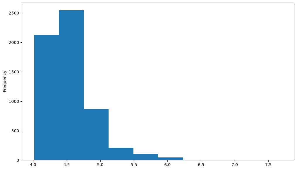
Before grouping, let’s get oriented — how many large events are in df, and what does the distribution of magnitudes look like?

len(df)

5923

df.mag.plot.hist()

<Axes: ylabel='Frequency'>

An Example

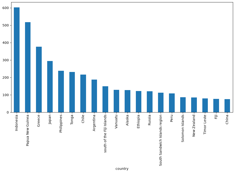
What if we wanted to know which country had the most earthquakes? groupby does this cleanly — it groups all rows that share a value, then we can apply an aggregation (here, count) to summarize each group:

df.groupby('country').mag.count().nlargest(20).plot(kind='bar', figsize=(12,6))

<Axes: xlabel='country'>

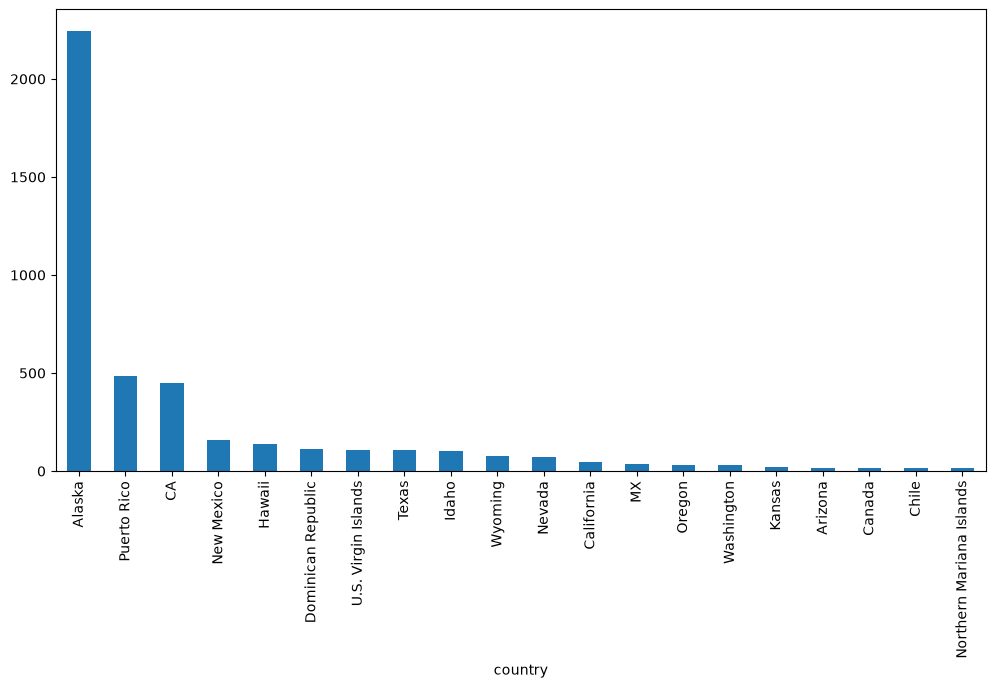
And the same count for the smaller events (df_small, magnitude below 4) — notice how the ranking of countries shifts:

df_small.groupby('country').mag.count().nlargest(20).plot(kind='bar', figsize=(12,6))

<Axes: xlabel='country'>

What Happened?

Let’s break down what groupby actually does. The .groupby(...) call doesn’t immediately compute anything — it returns a GroupBy object that holds the grouping logic. Computation happens when you call an aggregation method on it (.count(), .mean(), .aggregate(...), etc.). This pattern is sometimes called split-apply-combine:

1. Split the data into groups based on a column or function.

2. Apply a function (aggregate, transform, or filter) to each group independently.

3. Combine the results back into a single DataFrame or Series.

We can group by any Series — here, the country column itself:

df.country

id
us6000qkt1                            Tonga
us6000qksf                            Tonga
us6000qks2                      Philippines
us6000qkrz                           Russia
us6000qks0      southern Mid-Atlantic Ridge
                          ...              
us6000pll8                         Ethiopia
us6000pj3b                            Libya
us6000pj2q                            Tonga
us6000pll7    south of the Kermadec Islands
us6000plld                         Ethiopia
Name: country, Length: 5923, dtype: object

df.groupby(df.country)

<pandas.api.typing.DataFrameGroupBy object at 0x7f8f04d2ac10>

There is a shortcut for doing this with dataframes: you just pass the column name:

df.groupby('country')

<pandas.api.typing.DataFrameGroupBy object at 0x7f8f05043f10>

The GroupBy object

When we call groupby, we get back a GroupBy object:

gb = df.groupby('country')
gb

<pandas.api.typing.DataFrameGroupBy object at 0x7f8f059a26d0>

The length tells us how many groups were found:

len(gb)

194

All of the groups are available as a dictionary via the .groups attribute:

groups = gb.groups
len(groups)

194

groups.keys()

dict_keys(['2025 Drake Passage Earthquake', 'Afghanistan', 'Alaska', 'Algeria', 'Anguilla', 'Antigua and Barbuda', 'Arctic Ocean', 'Argentina', 'Armenia', 'Ascension Island region', 'Australia', 'Azerbaijan', 'Azores Islands region', 'Bahamas', 'Balleny Islands region', 'Banda Sea', 'Barbados', 'Bolivia', 'Bosnia and Herzegovina', 'Brazil', 'Burma', 'Burma (Myanmar)', 'Burma (Myanmar) Earthquake', 'CA', 'Canada', 'Carlsberg Ridge', 'Cayman Islands', 'Chad', 'Chagos Archipelago region', 'Chile', 'China', 'Colombia', 'Costa Rica', 'Croatia', 'Democratic Republic of the Congo', 'Dominica', 'Dominican Republic', 'Drake Passage', 'Easter Island region', 'Ecuador', 'Ecuador region', 'El Salvador', 'Eritrea', 'Ethiopia', 'Federated States of Micronesia', 'Federated States of Micronesia region', 'Fiji', 'Fiji region', 'Georgia', 'Greece', 'Greenland Sea', 'Guadeloupe', 'Guam', 'Guatemala', 'Hawaii', 'Honduras', 'Iceland', 'Iceland region', 'Idaho', 'India', 'India region', 'Indian Ocean Triple Junction', 'Indonesia', 'Iran', 'Italy', 'Japan', 'Japan region', 'Kazakhstan', 'Kermadec Islands region', 'Kuril Islands', 'Kuwait', 'Kyrgyzstan', 'Libya', 'MX', 'Macquarie Island region', 'Madagascar', 'Malawi', 'Mariana Islands region', 'Martinique', 'Mauritius', 'Mauritius - Reunion region', 'Mexico', 'Micronesia', 'Mid-Indian Ridge', 'Mongolia', 'Montenegro', 'Morocco', 'Nepal', 'New Caledonia', 'New Mexico', 'New Zealand', 'Nicaragua', 'North Atlantic Ocean', 'North Korea', 'Northern Mariana Islands', 'Norway', 'Norwegian Sea', 'Oman', 'Oregon', 'Owen Fracture Zone region', 'Pacific-Antarctic Ridge', 'Pakistan', 'Palau', 'Panama', 'Papua New Guinea', 'Peru', 'Philippines', 'Poland', 'Portugal', 'Prince Edward Islands region', 'Puerto Rico', 'Qatar', 'Revilla Gigedo Islands region', 'Reykjanes Ridge', 'Romania', 'Russia', 'Rwanda', 'Saint Helena', 'Saint Kitts and Nevis', 'Samoa', 'Saudi Arabia', 'Scotia Sea', 'Solomon Islands', 'Somalia', 'South Africa', 'South Atlantic Ocean', 'South Georgia Island region', 'South Indian Ocean', 'South Sandwich Islands region', 'South Shetland Islands', 'Southern Tibetan Plateau', 'Southwest Indian Ridge', 'Svalbard and Jan Mayen', 'Taiwan', 'Tajikistan', 'Tanzania', 'Tennessee', 'Texas', 'Thailand', 'Timor Leste', 'Tonga', 'Tristan da Cunha region', 'Tunisia', 'Turkey', 'U.S. Virgin Islands', 'Uganda', 'Ukraine', 'Uzbekistan', 'Vanuatu', 'Vanuatu region', 'Venezuela', 'Vietnam', 'Wallis and Futuna', 'Washington', 'West Chile Rise', 'Western Caribbean Sea', 'Xizang-Qinghai border region', 'Yemen', 'Zimbabwe', 'central East Pacific Rise', 'central Mid-Atlantic Ridge', 'east central Pacific Ocean', 'east of Severnaya Zemlya', 'east of the Kuril Islands', 'east of the South Sandwich Islands', 'north of Ascension Island', 'north of Franz Josef Land', 'north of Severnaya Zemlya', 'north of Svalbard', 'northern East Pacific Rise', 'northern Mid-Atlantic Ridge', 'northwest of New Zealand', 'northwest of the Kuril Islands', 'off the coast of Central America', 'off the coast of Ecuador', 'off the coast of Oregon', 'south of Africa', 'south of Panama', 'south of Tonga', 'south of the Fiji Islands', 'south of the Kermadec Islands', 'southeast Indian Ridge', 'southeast central Pacific Ocean', 'southeast of Easter Island', 'southeast of the Loyalty Islands', 'southern East Pacific Rise', 'southern Mid-Atlantic Ridge', 'southern Pacific Ocean', 'southwest of Africa', 'west of Macquarie Island', 'west of Vancouver Island', 'west of the Galapagos Islands', 'western Indian-Antarctic Ridge', 'western Xizang'])

list(groups.keys())

['2025 Drake Passage Earthquake',
 'Afghanistan',
 'Alaska',
 'Algeria',
 'Anguilla',
 'Antigua and Barbuda',
 'Arctic Ocean',
 'Argentina',
 'Armenia',
 'Ascension Island region',
 'Australia',
 'Azerbaijan',
 'Azores Islands region',
 'Bahamas',
 'Balleny Islands region',
 'Banda Sea',
 'Barbados',
 'Bolivia',
 'Bosnia and Herzegovina',
 'Brazil',
 'Burma',
 'Burma (Myanmar)',
 'Burma (Myanmar) Earthquake',
 'CA',
 'Canada',
 'Carlsberg Ridge',
 'Cayman Islands',
 'Chad',
 'Chagos Archipelago region',
 'Chile',
 'China',
 'Colombia',
 'Costa Rica',
 'Croatia',
 'Democratic Republic of the Congo',
 'Dominica',
 'Dominican Republic',
 'Drake Passage',
 'Easter Island region',
 'Ecuador',
 'Ecuador region',
 'El Salvador',
 'Eritrea',
 'Ethiopia',
 'Federated States of Micronesia',
 'Federated States of Micronesia region',
 'Fiji',
 'Fiji region',
 'Georgia',
 'Greece',
 'Greenland Sea',
 'Guadeloupe',
 'Guam',
 'Guatemala',
 'Hawaii',
 'Honduras',
 'Iceland',
 'Iceland region',
 'Idaho',
 'India',
 'India region',
 'Indian Ocean Triple Junction',
 'Indonesia',
 'Iran',
 'Italy',
 'Japan',
 'Japan region',
 'Kazakhstan',
 'Kermadec Islands region',
 'Kuril Islands',
 'Kuwait',
 'Kyrgyzstan',
 'Libya',
 'MX',
 'Macquarie Island region',
 'Madagascar',
 'Malawi',
 'Mariana Islands region',
 'Martinique',
 'Mauritius',
 'Mauritius - Reunion region',
 'Mexico',
 'Micronesia',
 'Mid-Indian Ridge',
 'Mongolia',
 'Montenegro',
 'Morocco',
 'Nepal',
 'New Caledonia',
 'New Mexico',
 'New Zealand',
 'Nicaragua',
 'North Atlantic Ocean',
 'North Korea',
 'Northern Mariana Islands',
 'Norway',
 'Norwegian Sea',
 'Oman',
 'Oregon',
 'Owen Fracture Zone region',
 'Pacific-Antarctic Ridge',
 'Pakistan',
 'Palau',
 'Panama',
 'Papua New Guinea',
 'Peru',
 'Philippines',
 'Poland',
 'Portugal',
 'Prince Edward Islands region',
 'Puerto Rico',
 'Qatar',
 'Revilla Gigedo Islands region',
 'Reykjanes Ridge',
 'Romania',
 'Russia',
 'Rwanda',
 'Saint Helena',
 'Saint Kitts and Nevis',
 'Samoa',
 'Saudi Arabia',
 'Scotia Sea',
 'Solomon Islands',
 'Somalia',
 'South Africa',
 'South Atlantic Ocean',
 'South Georgia Island region',
 'South Indian Ocean',
 'South Sandwich Islands region',
 'South Shetland Islands',
 'Southern Tibetan Plateau',
 'Southwest Indian Ridge',
 'Svalbard and Jan Mayen',
 'Taiwan',
 'Tajikistan',
 'Tanzania',
 'Tennessee',
 'Texas',
 'Thailand',
 'Timor Leste',
 'Tonga',
 'Tristan da Cunha region',
 'Tunisia',
 'Turkey',
 'U.S. Virgin Islands',
 'Uganda',
 'Ukraine',
 'Uzbekistan',
 'Vanuatu',
 'Vanuatu region',
 'Venezuela',
 'Vietnam',
 'Wallis and Futuna',
 'Washington',
 'West Chile Rise',
 'Western Caribbean Sea',
 'Xizang-Qinghai border region',
 'Yemen',
 'Zimbabwe',
 'central East Pacific Rise',
 'central Mid-Atlantic Ridge',
 'east central Pacific Ocean',
 'east of Severnaya Zemlya',
 'east of the Kuril Islands',
 'east of the South Sandwich Islands',
 'north of Ascension Island',
 'north of Franz Josef Land',
 'north of Severnaya Zemlya',
 'north of Svalbard',
 'northern East Pacific Rise',
 'northern Mid-Atlantic Ridge',
 'northwest of New Zealand',
 'northwest of the Kuril Islands',
 'off the coast of Central America',
 'off the coast of Ecuador',
 'off the coast of Oregon',
 'south of Africa',
 'south of Panama',
 'south of Tonga',
 'south of the Fiji Islands',
 'south of the Kermadec Islands',
 'southeast Indian Ridge',
 'southeast central Pacific Ocean',
 'southeast of Easter Island',
 'southeast of the Loyalty Islands',
 'southern East Pacific Rise',
 'southern Mid-Atlantic Ridge',
 'southern Pacific Ocean',
 'southwest of Africa',
 'west of Macquarie Island',
 'west of Vancouver Island',
 'west of the Galapagos Islands',
 'western Indian-Antarctic Ridge',
 'western Xizang']

Selecting and iterating over groups

The .groups attribute is a regular Python dictionary — its keys are the group labels and its values are the row indices in each group. You can look up a single group by name:

groups['Afghanistan']

Index(['us6000qkkm', 'us6000qjhm', 'us6000qiif', 'us6000qhyi', 'us6000qh0s',
       'us7000q1by', 'us7000q0z5', 'us7000q0aw', 'us7000q05h', 'us7000pzz5',
       'us7000pyne', 'us7000pydu', 'us7000px78', 'us7000pwle', 'us7000pve9',
       'us7000pvcr', 'us7000pv82', 'us7000pv7x', 'us7000pv02', 'us6000q76g',
       'us6000q6fr', 'us7000pw58', 'us6000q6c3', 'us7000ppcq', 'us7000pni6',
       'us7000pni0', 'us7000pne1', 'us7000pn0e', 'us7000pmym', 'us7000plhv',
       'us7000plec', 'us6000pzkp', 'us6000pxul', 'us6000pwru', 'us6000pxge',
       'us6000pvsk', 'us7000pflg', 'us7000pfcc', 'us7000pfc9', 'us7000pefx',
       'us7000pd3k', 'us7000pchv', 'us7000pb68', 'us7000pb30', 'us6000pmd7',
       'us6000plpp', 'us6000pk88', 'us6000pk23', 'us6000pjtx', 'us6000pjpy',
       'us6000pjlp'],
      dtype='str', name='id')

You can also loop over the groups directly. Each step of the loop gives you the group’s key and the sub-DataFrame of its rows:

for key, group in gb:
    display(group.head())
    print(f'The key is "{key}"')
    break

	time	latitude	longitude	depth	mag	magType	nst	gap	dmin	rms	...	place	type	horizontalError	depthError	magError	magNst	status	locationSource	magSource	country
id
us7000pwkn	2025-05-02 12:58:26.014000+00:00	-56.8094	-68.1019	10.0	7.4	mww	284.0	20.0	1.9	0.75	...	2025 Drake Passage Earthquake	earthquake	7.58	1.441	0.038	68.0	reviewed	us	us	2025 Drake Passage Earthquake

1 rows × 22 columns

The key is "2025 Drake Passage Earthquake"

Finally, you can pull out one group as its own DataFrame with get_group:

gb.get_group('Chile').head()

	time	latitude	longitude	depth	mag	magType	nst	gap	dmin	rms	...	place	type	horizontalError	depthError	magError	magNst	status	locationSource	magSource	country
id
us6000qkjt	2025-06-16 08:19:27.151000+00:00	-22.5784	-67.9279	172.967	4.4	mb	41.0	49.0	0.438	0.61	...	46 km NE of San Pedro de Atacama, Chile	earthquake	5.71	7.666	0.099	29.0	reviewed	us	us	Chile
us6000qkhr	2025-06-16 00:51:17.310000+00:00	-20.3278	-70.2485	41.960	4.4	mb	19.0	172.0	1.007	0.56	...	13 km WSW of La Tirana, Chile	earthquake	4.55	10.951	0.309	3.0	reviewed	us	us	Chile
us6000qkfl	2025-06-15 13:30:08.837000+00:00	-22.3399	-68.6815	117.138	4.3	mb	28.0	46.0	0.750	1.13	...	28 km ENE of Calama, Chile	earthquake	4.22	6.238	0.154	14.0	reviewed	us	us	Chile
us6000qjpw	2025-06-11 23:53:41.988000+00:00	-21.6724	-69.1225	98.543	4.1	mb	14.0	88.0	0.166	0.71	...	89 km NNW of Calama, Chile	earthquake	7.11	10.366	0.234	5.0	reviewed	us	us	Chile
us6000qj2v	2025-06-09 00:59:17.293000+00:00	-32.2490	-71.0761	83.965	4.1	mb	28.0	131.0	0.222	0.19	...	26 km NNE of La Ligua, Chile	earthquake	4.23	6.102	0.198	7.0	reviewed	us	us	Chile

5 rows × 22 columns

Try it

Take df. Use groupby to count the number of earthquakes per country and plot the top 10 as a bar chart (df.groupby('country').mag.count().nlargest(10).plot.bar()). Then use gb.get_group('Chile') to peek at the rows for a specific country.

Aggregation

Now that we know how to create a GroupBy object, let’s learn how to do aggregation on it.

One way is to use the .aggregate method, which accepts another function as its argument. The result is automatically combined into a new dataframe with the group key as the index.

gb.aggregate('max').head()

	time	latitude	longitude	depth	mag	magType	nst	gap	dmin	rms	...	updated	place	type	horizontalError	depthError	magError	magNst	status	locationSource	magSource
country
2025 Drake Passage Earthquake	2025-05-02 12:58:26.014000+00:00	-56.8094	-68.1019	10.000	7.4	mww	284.0	20.0	1.900	0.75	...	2025-06-06T12:21:50.736Z	2025 Drake Passage Earthquake	earthquake	7.58	1.441	0.038	68.0	reviewed	us	us
Afghanistan	2025-06-16 10:34:13.071000+00:00	37.4414	72.3551	230.241	5.7	mww	178.0	246.0	2.983	1.28	...	2025-06-16T11:33:01.040Z	80 km SSE of Farkhār, Afghanistan	earthquake	11.79	13.714	0.235	154.0	reviewed	us	us
Alaska	2025-06-14 14:32:06.018000+00:00	67.8223	178.6746	205.536	6.2	mww	287.0	219.0	2.579	1.37	...	2025-06-17T12:05:18.488Z	Rat Islands, Aleutian Islands, Alaska	earthquake	11.37	13.318	0.197	715.0	reviewed	us	us
Algeria	2025-03-18 09:50:26.946000+00:00	36.4349	3.4384	10.000	4.8	mww	167.0	55.0	3.516	0.51	...	2025-05-17T19:20:00.040Z	19 km SW of Lakhdaria, Algeria	earthquake	7.35	1.800	0.083	14.0	reviewed	us	us
Anguilla	2025-05-27 02:55:33.363000+00:00	19.3269	-63.1485	94.968	4.5	mb	75.0	138.0	1.427	0.72	...	2025-06-06T21:12:26.040Z	52 km NNW of Sandy Ground Village, Anguilla	earthquake	6.88	8.063	0.124	44.0	reviewed	us	us

5 rows × 21 columns

By default, the operation is applied to every column. That’s usually not what we want. We can use both . or [] syntax to select a specific column to operate on. Then we get back a series.

gb.mag

<pandas.api.typing.SeriesGroupBy object at 0x7f8f05051790>

gb.mag.aggregate('max')

country
2025 Drake Passage Earthquake     7.4
Afghanistan                       5.7
Alaska                            6.2
Algeria                           4.8
Anguilla                          4.5
                                 ... 
west of Macquarie Island          6.1
west of Vancouver Island          4.2
west of the Galapagos Islands     5.3
western Indian-Antarctic Ridge    6.2
western Xizang                    5.3
Name: mag, Length: 194, dtype: float64

gb.mag.aggregate('sum')

country
2025 Drake Passage Earthquake       7.4
Afghanistan                       221.7
Alaska                            583.3
Algeria                             4.8
Anguilla                           13.1
                                  ...  
west of Macquarie Island           75.3
west of Vancouver Island            4.2
west of the Galapagos Islands      46.1
western Indian-Antarctic Ridge    137.5
western Xizang                     40.5
Name: mag, Length: 194, dtype: float64

gb.mag.aggregate('mean')

country
2025 Drake Passage Earthquake     7.400000
Afghanistan                       4.347059
Alaska                            4.557031
Algeria                           4.800000
Anguilla                          4.366667
                                    ...   
west of Macquarie Island          4.706250
west of Vancouver Island          4.200000
west of the Galapagos Islands     4.610000
western Indian-Antarctic Ridge    4.741379
western Xizang                    4.500000
Name: mag, Length: 194, dtype: float64

gb.mag.aggregate('max').nlargest(10)

country
Burma (Myanmar) Earthquake       7.7
Cayman Islands                   7.6
2025 Drake Passage Earthquake    7.4
Tonga                            7.0
Papua New Guinea                 6.9
Reykjanes Ridge                  6.9
Japan                            6.8
Macquarie Island region          6.8
Burma (Myanmar)                  6.7
New Zealand                      6.7
Name: mag, dtype: float64

There are shortcuts for common aggregation functions:

gb.mag.max().nlargest(10)

country
Burma (Myanmar) Earthquake       7.7
Cayman Islands                   7.6
2025 Drake Passage Earthquake    7.4
Tonga                            7.0
Papua New Guinea                 6.9
Reykjanes Ridge                  6.9
Japan                            6.8
Macquarie Island region          6.8
Burma (Myanmar)                  6.7
New Zealand                      6.7
Name: mag, dtype: float64

gb.mag.min().nsmallest(10)

country
Puerto Rico            4.02
U.S. Virgin Islands    4.05
CA                     4.06
Dominican Republic     4.06
Afghanistan            4.10
Alaska                 4.10
Argentina              4.10
Australia              4.10
Bahamas                4.10
Bolivia                4.10
Name: mag, dtype: float64

gb.mag.mean().nlargest(10)

country
Burma (Myanmar) Earthquake            7.700000
2025 Drake Passage Earthquake         7.400000
Western Caribbean Sea                 5.400000
north of Franz Josef Land             5.300000
Macquarie Island region               5.233333
southeast central Pacific Ocean       5.200000
Morocco                               5.100000
Pacific-Antarctic Ridge               5.070588
South Atlantic Ocean                  5.050000
east of the South Sandwich Islands    5.000000
Name: mag, dtype: float64

gb.mag.std().nlargest(10)

country
Cayman Islands                    0.978713
U.S. Virgin Islands               0.909340
Macquarie Island region           0.895917
southwest of Africa               0.760263
Revilla Gigedo Islands region     0.726024
Svalbard and Jan Mayen            0.680241
India region                      0.643774
northwest of the Kuril Islands    0.643169
Panama                            0.621435
Reykjanes Ridge                   0.605769
Name: mag, dtype: float64

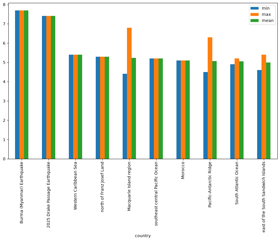
We can also apply multiple functions at once:

gb.mag.aggregate(['min', 'max', 'mean']).head()

	min	max	mean
country
2025 Drake Passage Earthquake	7.4	7.4	7.400000
Afghanistan	4.1	5.7	4.347059
Alaska	4.1	6.2	4.557031
Algeria	4.8	4.8	4.800000
Anguilla	4.2	4.5	4.366667

gb.mag.aggregate(['min', 'max', 'mean']).nlargest(10, 'mean').plot(kind='bar')

<Axes: xlabel='country'>

Try it

Group the earthquakes by country and use .aggregate(['min', 'max', 'mean']) on the mag column to get all three statistics at once. Then sort by the mean magnitude in descending order and grab the top 10 countries.

Transformation

The key difference between aggregation and transformation is that aggregation returns a smaller object than the original, indexed by the group keys, while transformation returns an object with the same index (and same size) as the original object. Groupby + transformation is used when applying an operation that requires information about the whole group.

In this example, we standardize the earthquakes in each country so that the distribution has zero mean and unit variance. We do this by first defining a function called standardize and then passing it to the transform method.

I admit that I don’t know why you would want to do this. transform makes more sense to me in the context of time grouping operation. See below for another example.

def standardize(x):
    return (x - x.mean())/x.std()

mag_standardized_by_country = gb.mag.transform(standardize)
mag_standardized_by_country.head()

id
us6000qkt1    0.668464
us6000qksf    0.419407
us6000qks2    2.157996
us6000qkrz    0.642692
us6000qks0    0.909743
Name: mag, dtype: float64

Try it

Define a function standardize(x) that returns (x - x.mean()) / x.std(). Use it with df.groupby('country').mag.transform(standardize) and plot a histogram of the result — magnitudes should now be approximately centered on zero within each country.

Time Grouping

We already saw how pandas has a strong built-in understanding of time. This capability is even more powerful in the context of groupby. With datasets indexed by a pandas DateTimeIndex, we can easily group and resample the data using common time units.

To get started, let’s load the timeseries data we already explored in past lessons.

import pooch
import pandas as pd

POOCH = pooch.create(
    path=pooch.os_cache("noaa-data"),
    base_url="doi:10.5281/zenodo.5553029/",
    registry={
        "HEADERS.txt": "md5:2a306ca225fe3ccb72a98953ded2f536",
        "CRND0103-2016-NY_Millbrook_3_W.txt": "md5:eb69811d14d0573ffa69f70dd9c768d9",
        "CRND0103-2017-NY_Millbrook_3_W.txt": "md5:b911da727ba1bdf26a34a775f25d1088",
        "CRND0103-2018-NY_Millbrook_3_W.txt": "md5:5b61bc687261596eba83801d7080dc56",
    },
)

with open(POOCH.fetch("HEADERS.txt")) as fp:
    headers = fp.read().split("\n")[1].split(" ")

dframes = []
for year in range(2016, 2019):
    fname = f"CRND0103-{year}-NY_Millbrook_3_W.txt"
    df = pd.read_csv(POOCH.fetch(fname), parse_dates=[1],
                     names=headers, header=None, sep=r"\s+",
                     na_values=[-9999.0, -99.0])
    dframes.append(df)

df = pd.concat(dframes)
df = df.set_index("LST_DATE")
df.head()

Downloading file 'HEADERS.txt' from 'doi:10.5281/zenodo.5553029/HEADERS.txt' to '/home/runner/.cache/noaa-data'.

Downloading file 'CRND0103-2016-NY_Millbrook_3_W.txt' from 'doi:10.5281/zenodo.5553029/CRND0103-2016-NY_Millbrook_3_W.txt' to '/home/runner/.cache/noaa-data'.

Downloading file 'CRND0103-2017-NY_Millbrook_3_W.txt' from 'doi:10.5281/zenodo.5553029/CRND0103-2017-NY_Millbrook_3_W.txt' to '/home/runner/.cache/noaa-data'.

Downloading file 'CRND0103-2018-NY_Millbrook_3_W.txt' from 'doi:10.5281/zenodo.5553029/CRND0103-2018-NY_Millbrook_3_W.txt' to '/home/runner/.cache/noaa-data'.

	WBANNO	CRX_VN	LONGITUDE	LATITUDE	T_DAILY_MAX	T_DAILY_MIN	T_DAILY_MEAN	T_DAILY_AVG	P_DAILY_CALC	SOLARAD_DAILY	...	SOIL_MOISTURE_10_DAILY	SOIL_MOISTURE_20_DAILY	SOIL_MOISTURE_50_DAILY	SOIL_MOISTURE_100_DAILY	SOIL_TEMP_5_DAILY	SOIL_TEMP_10_DAILY	SOIL_TEMP_20_DAILY	SOIL_TEMP_50_DAILY	SOIL_TEMP_100_DAILY
LST_DATE
2016-01-01	64756	2.422	-73.74	41.79	3.4	-0.5	1.5	1.3	0.0	1.69	...	0.233	0.204	0.155	0.147	4.2	4.4	5.1	6.0	7.6	NaN
2016-01-02	64756	2.422	-73.74	41.79	2.9	-3.6	-0.4	-0.3	0.0	6.25	...	0.227	0.199	0.152	0.144	2.8	3.1	4.2	5.7	7.4	NaN
2016-01-03	64756	2.422	-73.74	41.79	5.1	-1.8	1.6	1.1	0.0	5.69	...	0.223	0.196	0.151	0.141	2.6	2.8	3.8	5.2	7.2	NaN
2016-01-04	64756	2.422	-73.74	41.79	0.5	-14.4	-6.9	-7.5	0.0	9.17	...	0.220	0.194	0.148	0.139	1.7	2.1	3.4	4.9	6.9	NaN
2016-01-05	64756	2.422	-73.74	41.79	-5.2	-15.5	-10.3	-11.7	0.0	9.34	...	0.213	0.191	0.148	0.138	0.4	0.9	2.4	4.3	6.6	NaN

5 rows × 28 columns

This timeseries has daily resolution, and the daily plots are somewhat noisy.

df.T_DAILY_MEAN.plot()

<Axes: xlabel='LST_DATE'>

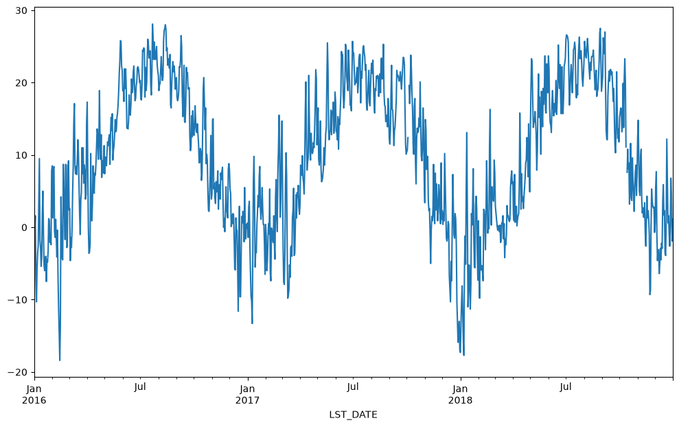
A common way to analyze such data in climate science is to create a “climatology,” which contains the average values in each month or day of the year. We can do this easily with groupby. Recall that df.index is a pandas DateTimeIndex object.

df.index

DatetimeIndex(['2016-01-01', '2016-01-02', '2016-01-03', '2016-01-04',
               '2016-01-05', '2016-01-06', '2016-01-07', '2016-01-08',
               '2016-01-09', '2016-01-10',
               ...
               '2018-12-22', '2018-12-23', '2018-12-24', '2018-12-25',
               '2018-12-26', '2018-12-27', '2018-12-28', '2018-12-29',
               '2018-12-30', '2018-12-31'],
              dtype='datetime64[us]', name='LST_DATE', length=1096, freq=None)

df.index.month

Index([ 1,  1,  1,  1,  1,  1,  1,  1,  1,  1,
       ...
       12, 12, 12, 12, 12, 12, 12, 12, 12, 12],
      dtype='int32', name='LST_DATE', length=1096)

monthly_climatology = df.select_dtypes(include='number').groupby(df.index.month).mean()
monthly_climatology

	WBANNO	CRX_VN	LONGITUDE	LATITUDE	T_DAILY_MAX	T_DAILY_MIN	T_DAILY_MEAN	T_DAILY_AVG	P_DAILY_CALC	SOLARAD_DAILY	...	SOIL_MOISTURE_10_DAILY	SOIL_MOISTURE_20_DAILY	SOIL_MOISTURE_50_DAILY	SOIL_MOISTURE_100_DAILY	SOIL_TEMP_5_DAILY	SOIL_TEMP_10_DAILY	SOIL_TEMP_20_DAILY	SOIL_TEMP_50_DAILY	SOIL_TEMP_100_DAILY
LST_DATE
1	64756.0	2.488667	-73.74	41.79	2.924731	-7.122581	-2.100000	-1.905376	2.478495	5.812258	...	0.240250	0.200717	0.153667	0.160880	0.150538	0.248387	0.788172	1.766667	3.364516	NaN
2	64756.0	2.487882	-73.74	41.79	6.431765	-5.015294	0.712941	1.022353	4.077647	8.495882	...	0.247771	0.210067	0.159176	0.163901	1.216471	1.169412	1.278824	1.617647	2.442353	NaN
3	64756.0	2.488667	-73.74	41.79	7.953763	-3.035484	2.455914	2.643011	2.788172	13.211290	...	0.228624	0.203634	0.157817	0.160366	3.450538	3.400000	3.372043	3.480645	3.777419	NaN
4	64756.0	2.488667	-73.74	41.79	14.793333	1.816667	8.302222	8.574444	2.396667	15.295889	...	0.214078	0.195844	0.153922	0.158100	9.415556	9.117778	8.455556	7.618889	6.670000	NaN
5	64756.0	2.488667	-73.74	41.79	21.235484	8.460215	14.850538	15.121505	3.015054	17.288602	...	0.204796	0.187097	0.148892	0.155720	16.934409	16.640860	15.612903	14.208602	12.455914	NaN
6	64756.0	2.488667	-73.74	41.79	25.627778	11.837778	18.733333	19.026667	3.053333	21.913333	...	0.136933	0.135211	0.129422	0.152722	22.403333	22.126667	20.956667	19.448889	17.552222	NaN
7	64756.0	2.488667	-73.74	41.79	28.568817	15.536559	22.054839	22.012903	3.865591	21.570645	...	0.105817	0.095204	0.114430	0.150014	25.448387	25.318280	24.163441	22.746237	21.068817	NaN
8	64756.0	2.488667	-73.74	41.79	27.473118	15.351613	21.410753	21.378495	4.480645	18.493333	...	0.156161	0.132333	0.128839	0.158800	24.758065	24.829032	24.116129	23.325806	22.301075	NaN
9	64756.0	2.488667	-73.74	41.79	24.084444	12.032222	18.057778	17.866667	3.730000	13.625667	...	0.136911	0.126456	0.121378	0.154000	21.028889	21.168889	20.921111	20.834444	20.707778	NaN
10	64756.0	2.548882	-73.74	41.79	18.127473	5.757143	11.938462	11.952747	3.228261	9.442527	...	0.155297	0.128473	0.120220	0.144618	14.872527	15.056044	15.379121	16.159341	17.059341	NaN
11	64756.0	2.555333	-73.74	41.79	9.586667	-1.375556	4.097778	4.277778	3.991111	6.350111	...	0.226111	0.212211	0.164789	0.163122	6.777778	6.975556	7.658889	9.048889	10.864444	NaN
12	64756.0	2.555333	-73.74	41.79	3.569892	-5.704301	-1.069892	-0.850538	2.791398	4.708602	...	0.259608	0.221301	0.171849	0.177194	1.831183	2.009677	2.647312	3.910753	5.710753	NaN

12 rows × 27 columns

monthly_climatology.T_DAILY_MAX.plot()

<Axes: xlabel='LST_DATE'>

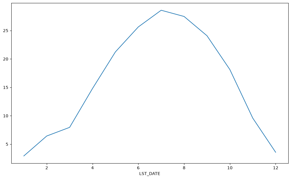
Each row in this new dataframe represents the average values for the months (1=January, 2=February, etc.)

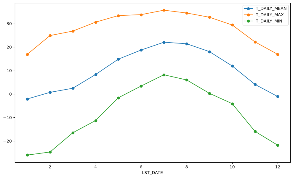
We can apply more customized aggregations, as with any groupby operation. Below we keep the mean of the mean, max of the max, and min of the min for the temperature measurements.

monthly_T_climatology = df.groupby(df.index.month).aggregate({'T_DAILY_MEAN': 'mean',
                                                              'T_DAILY_MAX': 'max',
                                                              'T_DAILY_MIN': 'min'})
monthly_T_climatology

	T_DAILY_MEAN	T_DAILY_MAX	T_DAILY_MIN
LST_DATE
1	-2.100000	16.9	-26.0
2	0.712941	24.9	-24.7
3	2.455914	26.8	-16.5
4	8.302222	30.6	-11.3
5	14.850538	33.4	-1.6
6	18.733333	33.8	3.4
7	22.054839	35.7	8.2
8	21.410753	34.5	6.0
9	18.057778	32.7	0.3
10	11.938462	29.4	-4.1
11	4.097778	22.2	-15.9
12	-1.069892	16.9	-21.8

monthly_T_climatology.plot(marker='o')

<Axes: xlabel='LST_DATE'>

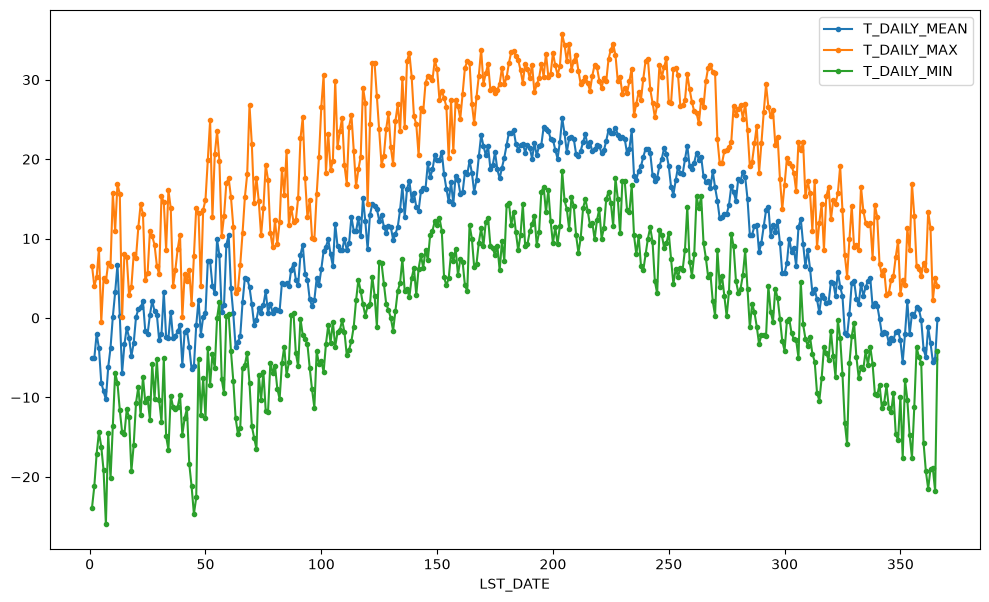
If we want to do it on a finer scale, we can group by day of year.

daily_T_climatology = df.groupby(df.index.dayofyear).aggregate({'T_DAILY_MEAN': 'mean',
                                                            'T_DAILY_MAX': 'max',
                                                            'T_DAILY_MIN': 'min'})
daily_T_climatology.plot(marker='.')

<Axes: xlabel='LST_DATE'>

Calculating anomalies

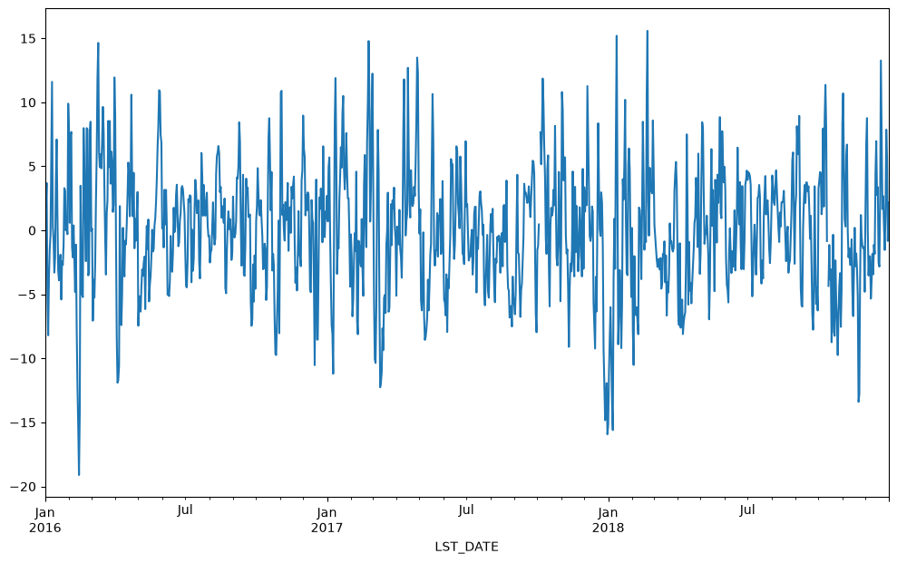
A common mode of analysis in climate science is to remove the climatology from a signal to focus only on the “anomaly” values. This can be accomplished with transformation.

def remove_climatology(x):
    return x - x.mean()

anomaly = df.groupby(df.index.month).T_DAILY_MEAN.transform(remove_climatology)
anomaly

LST_DATE
2016-01-01    3.600000
2016-01-02    1.700000
2016-01-03    3.700000
2016-01-04   -4.800000
2016-01-05   -8.200000
                ...   
2018-12-27    1.269892
2018-12-28    7.869892
2018-12-29    5.669892
2018-12-30   -0.830108
2018-12-31    2.169892
Name: T_DAILY_MEAN, Length: 1096, dtype: float64

anomaly.plot()

<Axes: xlabel='LST_DATE'>

Try it

Compute a daily climatology of T_DAILY_MEAN by grouping on df.index.dayofyear and taking the mean. Plot it as a line chart. Compare its shape to the monthly climatology shown above — the daily curve will be noisier but pick up sub-monthly structure.

Resampling

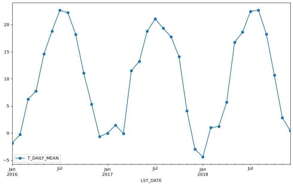
We met resample at the end of the previous notebook (Pandas Fundamentals) as a way to change a time series’ resolution. Now that we understand groupby, we can name what resample actually is: a groupby over time bins. Instead of grouping rows by the value in a column, it groups them by which time interval they fall into — each month, each year, and so on — then applies an aggregation. It’s the same split-apply-combine idea, just with time as the grouping key.

The bin size is given using pandas offset-alias syntax (e.g. 'ME' = month end, 'YE' = year end). Below we resample to a monthly frequency, taking the mean over each month.

df.select_dtypes(include='number').resample('ME').mean().plot(y='T_DAILY_MEAN', marker='o')

<Axes: xlabel='LST_DATE'>

df.select_dtypes(include='number').resample('ME').std().plot(y='T_DAILY_MEAN', marker='o')

<Axes: xlabel='LST_DATE'>

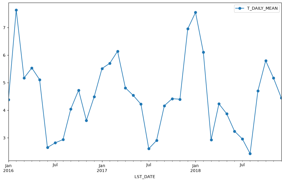
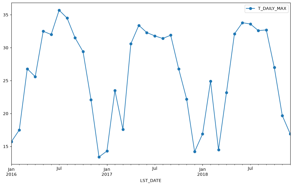
Just like with groupby, we can apply any aggregation function to our resample operation.

df.select_dtypes(include='number').resample('ME').max().plot(y='T_DAILY_MAX', marker='o')

<Axes: xlabel='LST_DATE'>

Try it

Use df.resample('YE').max() to get the yearly maximum and plot T_DAILY_MAX against the resulting yearly index. Compare with the monthly resampling shown above — what trend, if any, do you see?

Rolling Operations

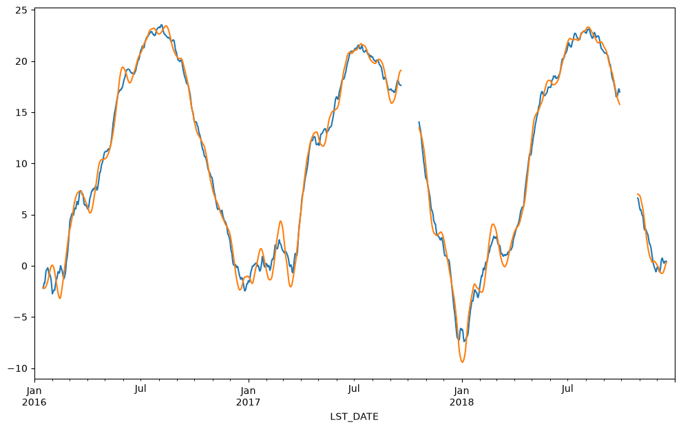
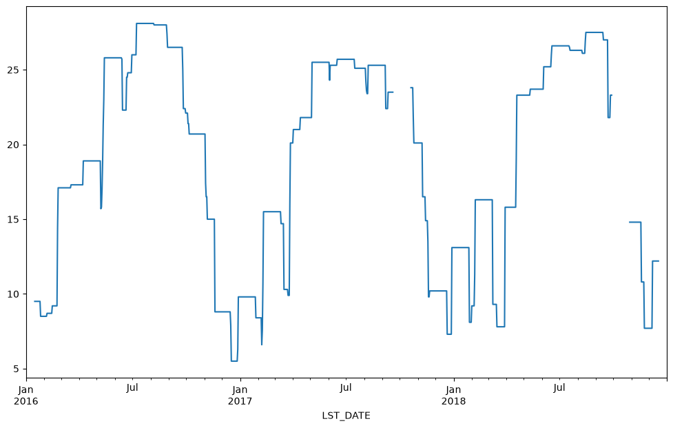
The final category of operations applies to “rolling windows”. (See rolling documentation.) We specify a function to apply over a moving window along the index. We specify the size of the window and, optionally, the weights. We also use the keyword center to tell pandas whether to center the operation around the midpoint of the window.

df.rolling(30, center=True).T_DAILY_MEAN.mean().plot()
df.rolling(30, center=True, win_type='triang').T_DAILY_MEAN.mean().plot()

<Axes: xlabel='LST_DATE'>

df.rolling(30, center=True).T_DAILY_MEAN.max().plot()

<Axes: xlabel='LST_DATE'>

Try it

Use df.rolling(7, center=True).T_DAILY_MEAN.mean() to compute a 7-day moving average and plot it. Then overlay the raw daily series on the same axes (call .plot() twice on the same axes, or use fig, ax = plt.subplots() and call .plot(ax=ax) for each). What does smoothing reveal that the raw data hides?

Recap

This notebook was all about split–apply–combine:

• groupby on a column — grouping earthquakes by country, then summarizing each group with aggregation (count, mean, .aggregate([...])).

• Transformation — returning a value for every row using whole-group information (standardizing within each group; removing a climatology to get anomalies).

• Time grouping — grouping by parts of a DatetimeIndex to build a climatology.

• resample — a groupby over time bins, for changing time resolution.

• rolling — moving-window calculations for smoothing.

These same groupby / resample / rolling ideas carry straight into the next section, Xarray, where they work on labelled N-dimensional arrays.