
Assignment 4a: NumPy and Matplotlib#
At-home assignment — worth 10 points. When you’re done, push your work to your week folder and post a link to your completed notebook on the matching Courseworks assignment.
The goal of this assignment is to gain comfort creating, visualizing, and computing with numpy arrays.
Learning goals
This assignment exercises the scientific Python skills from this section:
Create new arrays using
linspaceandarangeCompute formulas with numpy arrays (element-wise math + broadcasting)
Load data from
.npyfilesUse reductions (
mean,std,nanmean,nanstd) along specific axesMake 1D line plots, scatter plots, and add titles / axis labels
Working through this notebook
Download this notebook using the ⬇ button in the top-right (or copy-paste the cells into a fresh notebook), open it in your environment (JupyterLab on LEAP or Colab), and fill in your solution under each numbered task.
When you’re done, follow the submission instructions at the bottom of the page.
Part 1: Creating and Manipulating Arrays#
Start by importing numpy (as np) and matplotlib’s pyplot (as plt). The cell below is empty — type your imports there and run it.
1.1. Create two 2D arrays representing coordinates x, y on the cartesian plan#
Both should cover the range (-2, 2) and have 100 points in each direction
1.2. Visualize each 2D array using pcolormesh#
Use the correct coordinates for the x and y axes.
1.3 Compute a smooth 2D field and plot it#
Using your x and y arrays, compute the Gaussian “hill”
(use np.exp(...)). Then plot f on the \(x\)/\(y\) plane with pcolormesh and add a colorbar.
1.4 Plot the mean of f over the x-axis#
Average f across the x-direction (f.mean(axis=...)) so you’re left with a 1D profile as a function of y. Plot it.
1.5 Plot the mean of f over the y-axis#
Now average across the y-direction instead, leaving a profile as a function of x. Plot it.
Part 2: Analyze ARGO Data#
In this problem, we use real data from ocean profiling floats. ARGO floats are autonomous robotic instruments that collect Temperature, Salinity, and Pressure data from the ocean. ARGO floats collect one “profile” (a set of messurements at different depths or “levels”).
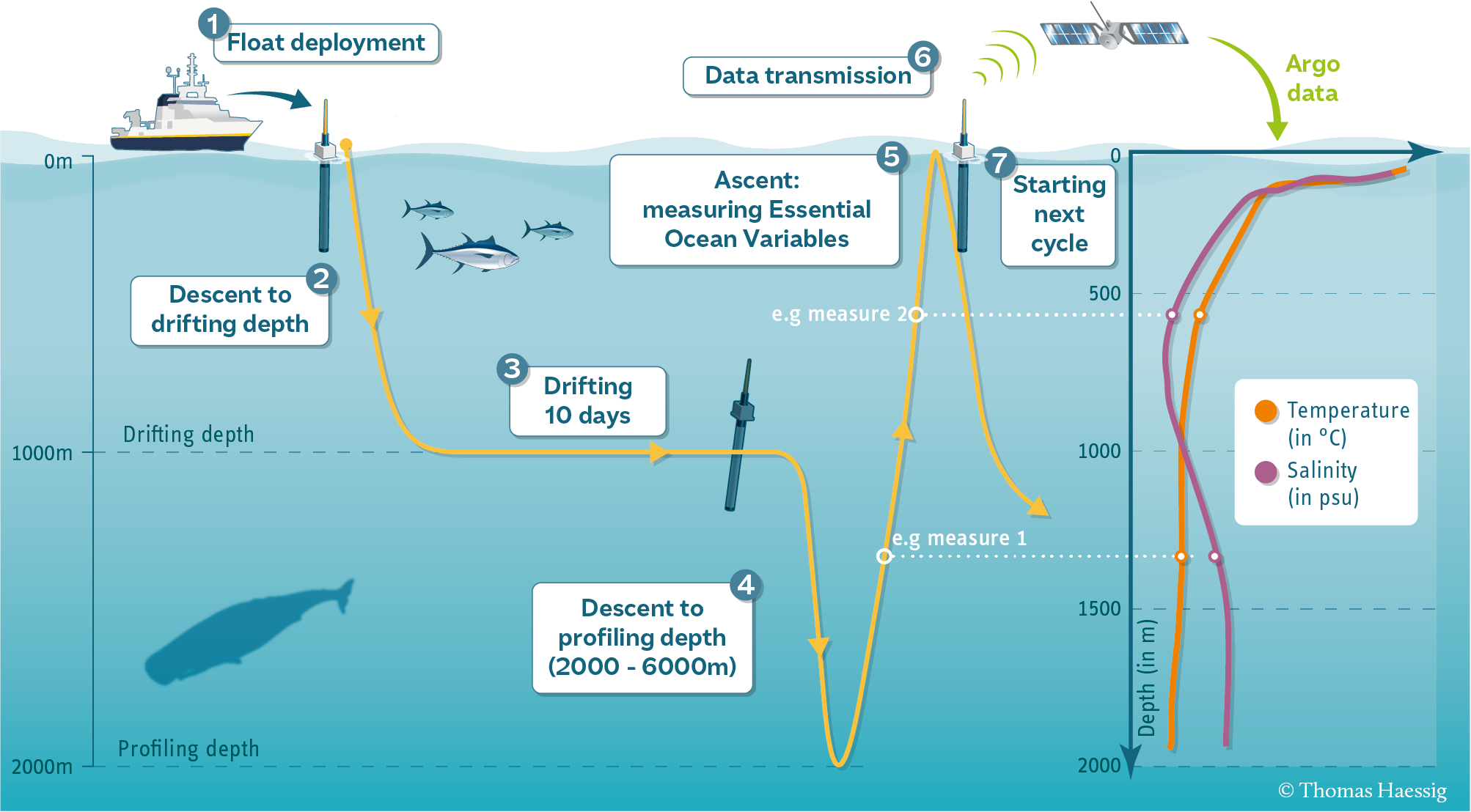
Each profile has a single latitude, longitude, and date associated with it, in addition to many different levels.
Let’s start by using pooch to download the data files we need for this exercise.
The following code will give you a list of .npy files that you can open in the next step.
import pooch
url = "https://github.com/earth-DS-ML/summer_2026/raw/refs/heads/main/assignments/more_matplotlib_data/argo_data_example.zip"
files = pooch.retrieve(url, processor=pooch.Unzip(), known_hash="650948c4b84690d370ad6f8aa9279c165f5302d3d9a7d330d3c0232b9d244e13")
files
2.1 Load each data file as a numpy array.#
You can use whatever names you want for your arrays, but I recommend
T: temperature
S: salinity
P: pressure
date: date
lat: latitude
lon: longitude
level: depth level
Note: you have to actually look at the file name (the items in files) to know which files corresponds to which variable.
2.3 Make a plot for each column of data in T, S and P (three plots).#
The vertical scale should be the levels data. Each plot should have a line for each column of data. It will look messy.
2.4 Compute the mean and standard deviation of each of T, S and P at each depth in level.#
2.5 Now make three similar plot, but show only the mean T, S and P at each depth. Show error bars on each plot using the standard deviations.#
2.6 Account For Missing Data#
The profiles contain many missing values. These are indicated by the special “Not a Number” value, or np.nan.
When you take the mean or standard deviation of data with NaNs in it, the entire result becomes NaN. Instead, if you use the special functions np.nanmean and np.nanstd, you tell NumPy to ignore the NaNs.
Recalculate the means and standard deviations as in the previous sections using these functions and plot the results.
2.7 Create a scatter plot of the lon, lat positions of the ARGO float.#
Use the plt.scatter function.
Submission instructions#
When you’re done, save your completed notebook as assignment4a.ipynb inside the current week’s folder (e.g. week4/) in your private clmt5405-assignments GitHub repo. Then push the commit:
git add <weekN>/assignment4a.ipynb
git commit -m "Submit assignment 4a"
git push
Due Sunday night.