
Overview#
In the previous module, we saw how Pandas keeps track of the “metadata” surrounding tabular datasets — an index for each row and labels for each column. These features, together with Pandas’ many routines for data munging and analysis, have made it one of the most popular Python packages in the world.
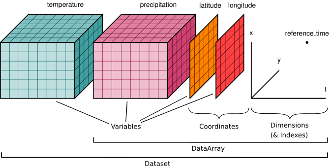
However, not all Earth and environmental datasets fit the “tabular” (rows-and-columns) model. We often deal with multidimensional data (also called N-dimensional): data with many independent dimensions or axes. For example, we might represent Earth’s surface temperature \(T\) as a three-dimensional variable
where \(x\) is longitude, \(y\) is latitude, and \(t\) is time.
Xarray brings pandas-level convenience to this kind of labelled, multidimensional data — and it is the workhorse for gridded climate data, from model output and reanalysis to satellite fields.
Learning objectives#
Because xarray is central to gridded-data analysis in the Earth and environmental sciences, we give it a full section. By the end you should be able to:
Lesson 1: Xarray Fundamentals#
Dataset Creation#
Describe the core xarray data structures, the
DataArrayand theDataset, and the components that make them up, including: Data Variables, Dimensions, Coordinates, Indexes, and AttributesCreate xarray
DataArraysandDatasetsout of raw numpy arraysCreate xarray objects with and without indexes
Load xarray datasets from netCDF files and OPeNDAP servers
View and set attributes
Basic Indexing and Interpolation#
Select data by position using
.iselwith values or slicesSelect data by label using
.selwith values or slicesSelect timeseries data by date/time with values or slices
Use nearest-neighbor lookups with
.selMask data with
.whereInterpolate data in one and several dimensions
Basic Computation#
Do basic arithmetic with DataArrays and Datasets
Use numpy universal functions on DataArrays and Datasets, or use corresponding built-in xarray methods
Combine multiple xarray objects in arithmetic operations and understand how they are broadcast / aligned
Perform aggregation (reduction) along one or multiple dimensions of a DataArray or Dataset
Basic Plotting#
Use built-in xarray plotting for 1D and 2D DataArrays
Customize plots with options
Lesson 2: Advanced Usage#
Xarray’s groupby, resample, and rolling#
Split xarray objects into groups using
groupbyApply reduction operations to groups (e.g. mean)
Apply non-reducing functions to groups (e.g. standardize)
Use
groupbywith time coordinates (e.g. to create climatologies)Use arithmetic between
GroupByobjects and regular DataArrays / DatasetsUse
groupby_binsto aggregate data in binsUse
resampleon time dimensionsUse
rollingto apply rolling aggregations
Merging and Combining Datasets#
Concatenate DataArrays and Datasets along a new or existing dimension
Merge multiple datasets with different variables
Add a new data variable to an existing Dataset
Reshaping Data#
Transpose dimension order
Swap coordinates
Expand and squeeze dimensions
Convert between DataArray and Dataset
Use
stackandunstackto transform data
Advanced Computations#
Use
differentiateto take derivatives of dataUse
apply_ufuncto apply custom or specialized operations to data
Pages in this section#
Xarray Fundamentals — DataArrays and Datasets, label-based selection, computation, broadcasting, reductions, and loading netCDF/Zarr data.
Xarray: Advanced — interpolation,
groupby,resample,rolling, andcoarsen; building climatologies and more.Assignment 6: Xarray with SST data — apply xarray to NOAA sea-surface-temperature data (the at-home assignment).
In-class assignment — 10 points
Your in-class assignment for this section is to complete the “Try it” exercises in the lecture notebooks above. Work through them in your own copy of each notebook. To submit, push your completed notebook(s) to your week folder and post a link to each on the matching Courseworks assignment. (The at-home assignment — Assignment 6, the SST lab — is graded separately, 10 points.)
Working through the lectures#
Same workflow as previous modules — download each notebook (⬇ icon, top-right) or copy-paste the cells into a fresh notebook in JupyterLab on LEAP or Colab, then step through them. Stop at each Try it admonition to experiment in your own cells before moving on.