Assignment 6: Xarray with Sea Surface Temperature (SST) data

Assignment 6: Xarray with Sea Surface Temperature (SST) data#

At-home assignment — worth 10 points. When you’re done, push your work to your week folder and post a link to your completed notebook on the matching Courseworks assignment.

In this lab you’ll apply xarray to NOAA’s Extended Reconstructed SST (ERSST v5) dataset, accessed over OPeNDAP:

https://psl.noaa.gov/thredds/dodsC/Datasets/noaa.ersst.v5/sst.mnmean.nc

Learning goals

This assignment exercises the xarray skills from this section:

Open a gridded dataset over OPeNDAP and inspect its metadata (attrs, long_name)
Compute time-means and spatial means; plot maps and timeseries
Build a latitude (\(\cos\lambda\)) weighting and take an area-weighted spatial mean
Select point locations with .sel and combine them along a new location dimension with concat
Use groupby to build a climatology and anomalies, and rolling for a running mean
Compute the Niño 3.4 ENSO index from SST anomalies

Working through this notebook

Download this notebook using the ⬇ button in the top-right (or copy-paste the cells into a fresh notebook), open it in your environment (JupyterLab on LEAP or Colab), and fill in your solution under each numbered task.

When you’re done, follow the submission instructions at the bottom of the page.

Start by importing NumPy, Matplotlib, and Xarray. Set the default figure size to (12, 6).

1) Opening data and examining the metadata#

1.1) Open the dataset and display its contents#

Heads up — open this dataset with chunks

This OPeNDAP server quietly returns all zeros (you’ll get blank maps and flat timeseries) if you request the whole array in a single shot — which several tasks below do (the time-mean in 2.1, the spatial mean in 2.3, the ENSO index in part 4). Avoid it by opening the data in pieces with Dask, so xarray fetches it chunk-by-chunk:

ds = xr.open_dataset(url, chunks={'time': 120})

Everything else works exactly as usual — reductions like .mean() pull the data in as needed. (You can combine this with other keywords, e.g. drop_variables=['time_bnds'].)

1.2) Print out the `long_name` attribute of each variable and coordinate#

2) Basic reductions, arithmetic, means, and plotting#

2.1) Calculate the time-mean of the entire dataset#

2.2) Plot a map of the time-mean that was generated in the above part#

2.3) Calculate a spatial mean for each time, and plot this as a timeseries#

2.4) Create a `weight` array proportional to \(\cos(\lambda)\)#

Think carefully a about radians vs. degrees

The goal here is to realize that the dataset is provided on a \(2^o\)X\(2^o\) lat-lon grid. But we know that the distance between longitude lines shrinks as we approach the poles.

This means that if we take a naive mean (as done in the above part), we are overemphasizing the influence of the regions away from the equator (since their area is smaller but they contribute the same to the mean). So here we plan to appropriately weight our data.

2.5) Redo the calculation of the spatial mean for each time, and plot this as a timeseries#

3) Selecting and Merging Data#

For the next problem, use the following approximate locations of four different locations in the ocean.

city	lon	lat
Equatorial Pacific (EP)	250 E	0 N
Southern Ocean (SO)	50 E	60 S
North Atlantic (NAtl)	300 E	30 N
Arabian Sea (AS)	60 E	20 N

3.1) Create a dataset for each point from the global dataset#

3.2) Combine these four datasets into a new dataset with the new dimension `location`#

Create a new dimension coordinate to hold the location name. Display the combined dataset.

3.3) Plot the SST at each location as a timeseries over the last 3 years#

4) Group by and ENSO: Reproduce the SST curve from the figure below#

enso

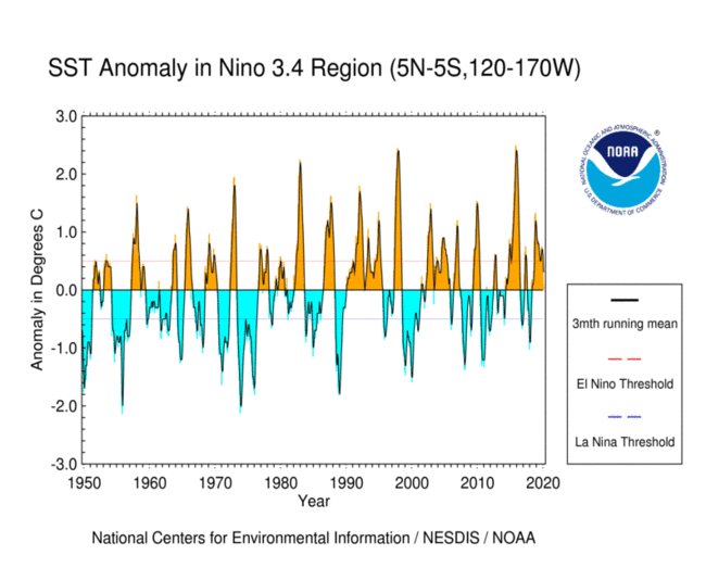
You don’t have to match the stylistic details, or use different colors above and below zero, just the “3mth running mean” curve.

Here will will calculate the NINO 3.4 index of El Nino variabillity (which is the quantity shown in the above plot) and use it to analyze datasets.

The Niño 3.4 region is defined as the region between +/- 5 deg. lat, 170 W - 120 W lon.
Warm or cold phases of the Oceanic Niño Index are defined by a five consecutive 3-month running mean of sea surface temperature (SST) anomalies in the Niño 3.4 region that is above the threshold of +0.5°C (warm), or below the threshold of -0.5°C (cold). This is known as the Oceanic Niño Index (ONI).

(Note that “anomaly” means that the seasonal cycle, also called the “climatology” has been removed.)

Also for this part: Drop the time_bnds variable as we did in class and trim the data to 1950 onward for this assignment.

Submission instructions#

When you’re done, save your completed notebook as assignment6.ipynb inside the current week’s folder in your private clmt5405-assignments GitHub repo, then push the commit:

git add <weekN>/assignment6.ipynb
git commit -m "Submit the Xarray SST lab"
git push

Then post a link to your completed notebook on the matching Courseworks assignment. Due Sunday night.