Pandas Fundamentals

Working through this notebook

This page is a Jupyter notebook. Download it using the ⬇ button in the top-right (or copy-paste the cells into a fresh notebook), open it in your environment (JupyterLab on LEAP or Colab), and step through the cells. When you reach a Try it admonition, experiment in your own cells before moving on.

In-class assignment — 10 points

The “Try it” exercises in this notebook are part of your in-class assignment for this section. Complete them in your own copy of the notebook, push it to your week folder, and post the notebook link on the matching Courseworks assignment. (One 10-point assignment covers all the lecture notebooks in this section.)

Let’s start by importing the libraries we’ll use throughout this lecture: pandas (conventionally imported as pd), NumPy, and matplotlib’s pyplot.

import pandas as pd
import numpy as np
from matplotlib import pyplot as plt
%matplotlib inline

Series

Pandas gives you two main objects to work with: a Series (one-dimensional, like a single column of labelled data) and a DataFrame (two-dimensional, like a table or spreadsheet). DataFrames are built up from Series — each column of a DataFrame is itself a Series — so we’ll start with Series and then build up to DataFrame.

A Series is a one-dimensional array of data with an index: labels we use to access each value.

There are many ways to create a Series. Let’s start with a simple example using planet names and masses.

To create a Series, we pass two lists to pd.Series(...): the data values, and an index containing the labels for those values. The output below will show the labels on the left and the values on the right:

names = ['Mercury', 'Venus', 'Earth']
values = [0.3e24, 4.87e24, 5.97e24]
masses = pd.Series(values, index=names)
masses

Mercury    3.000000e+23
Venus      4.870000e+24
Earth      5.970000e+24
dtype: float64

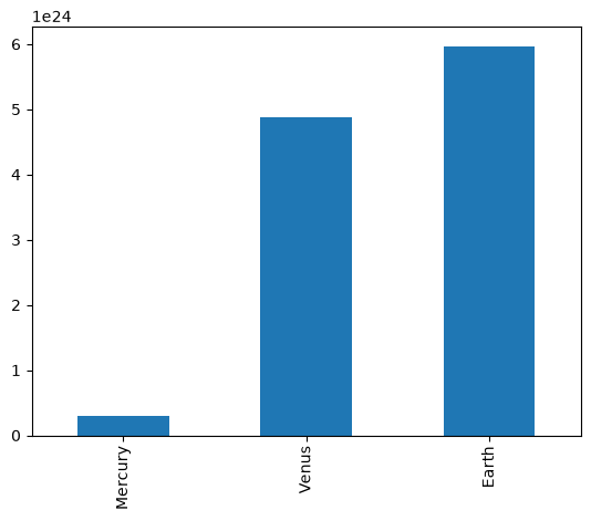
Series have built in plotting methods.

masses.plot(kind='bar')

<Axes: >

Arithmetic operations and most numpy function can be applied to Series. An important point is that the Series keep their index during such operations.

np.log(masses) / masses**2

Mercury    6.006452e-46
Venus      2.396820e-48
Earth      1.600655e-48
dtype: float64

We can access the underlying index object if we need to:

masses.index

Index(['Mercury', 'Venus', 'Earth'], dtype='str')

Indexing

We can get values back out using the index via the .loc attribute

masses.loc['Earth']

np.float64(5.97e+24)

Or by raw position using .iloc

masses.iloc[2]

np.float64(5.97e+24)

We can pass a list or array to loc to get multiple rows back:

masses.loc[['Venus', 'Earth']]

Venus    4.870000e+24
Earth    5.970000e+24
dtype: float64

And we can even use slice notation

masses.loc['Mercury':'Earth']

Mercury    3.000000e+23
Venus      4.870000e+24
Earth      5.970000e+24
dtype: float64

masses.iloc[:2]

Mercury    3.000000e+23
Venus      4.870000e+24
dtype: float64

If we need to, we can always get the raw data back out as well

masses.values # a numpy array

array([3.00e+23, 4.87e+24, 5.97e+24])

masses.index # a pandas Index object

Index(['Mercury', 'Venus', 'Earth'], dtype='str')

Try it

In a fresh code cell, build your own Series from a Python list of values and a list of labels (any topic of your choice — e.g., capital cities mapped to populations). Use .loc[] to access one element by label, and .iloc[] to access the same element by position. Then slice with .loc[] over a label range — note that both the start and end labels are included (unlike Python list slicing).

DataFrame

There is a lot more to Series, but they are limited to a single “column”. A more useful Pandas data structure is the DataFrame. A DataFrame is basically a bunch of series that share the same index. It’s a lot like a table in a spreadsheet.

Below we create a DataFrame.

Now let’s build a DataFrame. The most common pattern is to start with a Python dictionary mapping column names to lists of values, then pass it to pd.DataFrame:

data = {'mass': [0.3e24, 4.87e24, 5.97e24],       # kg
        'diameter': [4879e3, 12_104e3, 12_756e3], # m
        'rotation_period': [1407.6, np.nan, 23.9] # h
       }
df = pd.DataFrame(data, index=['Mercury', 'Venus', 'Earth'])
df

	mass	diameter	rotation_period
Mercury	3.000000e+23	4879000.0	1407.6
Venus	4.870000e+24	12104000.0	NaN
Earth	5.970000e+24	12756000.0	23.9

Pandas handles missing data very elegantly, keeping track of it through all calculations.

DataFrames come with a lot of built-in inspection and summary methods. A few of the most useful:

df.info()

<class 'pandas.DataFrame'>
Index: 3 entries, Mercury to Earth
Data columns (total 3 columns):
 #   Column           Non-Null Count  Dtype  
---  ------           --------------  -----  
 0   mass             3 non-null      float64
 1   diameter         3 non-null      float64
 2   rotation_period  2 non-null      float64
dtypes: float64(3)
memory usage: 96.0+ bytes

A wide range of statistical functions are available on both Series and DataFrames.

df.min()

mass               3.000000e+23
diameter           4.879000e+06
rotation_period    2.390000e+01
dtype: float64

df.mean()

mass               3.713333e+24
diameter           9.913000e+06
rotation_period    7.157500e+02
dtype: float64

df.std()

mass               3.006765e+24
diameter           4.371744e+06
rotation_period    9.784237e+02
dtype: float64

df.describe()

	mass	diameter	rotation_period
count	3.000000e+00	3.000000e+00	2.000000
mean	3.713333e+24	9.913000e+06	715.750000
std	3.006765e+24	4.371744e+06	978.423653
min	3.000000e+23	4.879000e+06	23.900000
25%	2.585000e+24	8.491500e+06	369.825000
50%	4.870000e+24	1.210400e+07	715.750000
75%	5.420000e+24	1.243000e+07	1061.675000
max	5.970000e+24	1.275600e+07	1407.600000

We can get a single column as a Series using python’s getitem syntax on the DataFrame object.

df['mass']

Mercury    3.000000e+23
Venus      4.870000e+24
Earth      5.970000e+24
Name: mass, dtype: float64

…or using attribute syntax.

df.mass

Mercury    3.000000e+23
Venus      4.870000e+24
Earth      5.970000e+24
Name: mass, dtype: float64

Try it

Build your own DataFrame from a dictionary of columns (any topic — e.g. a few cities with population, area, and elevation), passing an index of labels. Include at least one np.nan so you can see how pandas reports missing data. Inspect its structure with .info() and .describe(), then compute a few summary statistics with .mean(), .min(), and .std() — try them on the whole DataFrame and on a single column (e.g. df['population'].mean()). Finally, pull a column out as a Series using both df['col'] and df.col.

Indexing works very similar to series

df.loc['Earth']

mass               5.970000e+24
diameter           1.275600e+07
rotation_period    2.390000e+01
Name: Earth, dtype: float64

df.iloc[2]

mass               5.970000e+24
diameter           1.275600e+07
rotation_period    2.390000e+01
Name: Earth, dtype: float64

But we can also specify the column we want to access

df.loc['Earth', 'mass']

np.float64(5.97e+24)

df.iloc[:2, 0]

Mercury    3.000000e+23
Venus      4.870000e+24
Name: mass, dtype: float64

If we make a calculation using columns from the DataFrame, it will keep the same index:

volume =  4/3 * np.pi * (df.diameter/2)**3
df.mass / volume

Mercury    4933.216530
Venus      5244.977070
Earth      5493.285577
dtype: float64

Which we can easily add as another column to the DataFrame:

df['density'] = df.mass / volume
df

	mass	diameter	rotation_period	density
Mercury	3.000000e+23	4879000.0	1407.6	4933.216530
Venus	4.870000e+24	12104000.0	NaN	5244.977070
Earth	5.970000e+24	12756000.0	23.9	5493.285577

Merging Data

Pandas supports a wide range of methods for merging different datasets. These are described extensively in the documentation. Here we just give a few examples.

Pandas can merge DataFrames and Series intelligently along their shared index. Let’s create a separate Series of planet temperatures and combine it with our existing DataFrame:

temperature = pd.Series([167, 464, 15, -65],
                     index=['Mercury', 'Venus', 'Earth', 'Mars'],
                     name='temperature')
temperature

Mercury    167
Venus      464
Earth       15
Mars       -65
Name: temperature, dtype: int64

df.join(temperature)

	mass	diameter	rotation_period	density	temperature
Mercury	3.000000e+23	4879000.0	1407.6	4933.216530	167
Venus	4.870000e+24	12104000.0	NaN	5244.977070	464
Earth	5.970000e+24	12756000.0	23.9	5493.285577	15

By default, join keeps the calling DataFrame’s index — a left join — so Mars is dropped, since it isn’t one of our three planets. The how keyword changes this: how='right' keeps the other object’s index instead, so Mars appears (with NaN for the columns we don’t have for it):

df.join(temperature, how='right')

	mass	diameter	rotation_period	density	temperature
Mercury	3.000000e+23	4879000.0	1407.6	4933.216530	167
Venus	4.870000e+24	12104000.0	NaN	5244.977070	464
Earth	5.970000e+24	12756000.0	23.9	5493.285577	15
Mars	NaN	NaN	NaN	NaN	-65

reindex is a more general tool: it conforms a DataFrame to a brand-new index that you supply, inserting rows of NaN wherever a label wasn’t already present:

everyone = df.reindex(['Mercury', 'Venus', 'Earth', 'Mars'])
everyone

	mass	diameter	rotation_period	density
Mercury	3.000000e+23	4879000.0	1407.6	4933.216530
Venus	4.870000e+24	12104000.0	NaN	5244.977070
Earth	5.970000e+24	12756000.0	23.9	5493.285577
Mars	NaN	NaN	NaN	NaN

Try it

Create a new Series of values indexed by some of the planets — you can include one that isn’t in the DataFrame (e.g. Mars or Jupiter) — and join it onto the planets DataFrame. Try how='right' and compare the result with the default join. Then call .reindex(...) with your own list of planet names and notice how pandas fills in NaN for labels that weren’t present.

Another powerful way to select data is to pick rows based on a condition rather than by their label or position. A comparison like df.mass > 4e24 is checked for every row and returns a boolean Series — a column of True/False values, one per planet. Placing that inside df[...] keeps only the rows where the value is True. For example, to get just the planets more massive than 4e24 kg:

adults = df[df.mass > 4e24]
adults

	mass	diameter	rotation_period	density
Venus	4.870000e+24	12104000.0	NaN	5244.977070
Earth	5.970000e+24	12756000.0	23.9	5493.285577

Since that condition is itself just a Series of True/False values, we can also store it as a new column — a handy way to flag the rows that meet the criterion:

df['is_big'] = df.mass > 4e24
df

	mass	diameter	rotation_period	density	is_big
Mercury	3.000000e+23	4879000.0	1407.6	4933.216530	False
Venus	4.870000e+24	12104000.0	NaN	5244.977070	True
Earth	5.970000e+24	12756000.0	23.9	5493.285577	True

Modifying Values

We often want to modify values in a dataframe based on some rule. To modify values, we need to use .loc or .iloc

df.loc['Earth', 'mass'] = 5.98e+24
df.loc['Venus', 'diameter'] += 1
df

	mass	diameter	rotation_period	density	is_big
Mercury	3.000000e+23	4879000.0	1407.6	4933.216530	False
Venus	4.870000e+24	12104001.0	NaN	5244.977070	True
Earth	5.980000e+24	12756000.0	23.9	5493.285577	True

Try it

Take the planets DataFrame from above. Use .loc[] to get all of Earth’s data, then .iloc[:3] to get the first three rows. Add a new column called density_check computed as df.mass / (4/3 * np.pi * (df.diameter/2)**3), then filter the DataFrame to planets with mass greater than 1e24.

Plotting

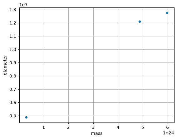
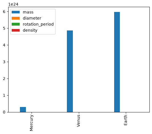
DataFrames have all kinds of useful plotting built in.

df.plot(kind='scatter', x='mass', y='diameter', grid=True)

<Axes: xlabel='mass', ylabel='diameter'>

df.plot(kind='bar')

<Axes: >

Try it

Make a scatter plot of diameter vs mass from the planets DataFrame. Then make a bar chart of each planet’s mass. (You can stay with df.plot(kind='...'), or use df.plot.scatter(...) / df.plot.bar(...) — both work.)

Time Indexes

Indexes are very powerful. They are a big part of why Pandas is so useful. There are different indices for different types of data. Time Indexes are especially great!

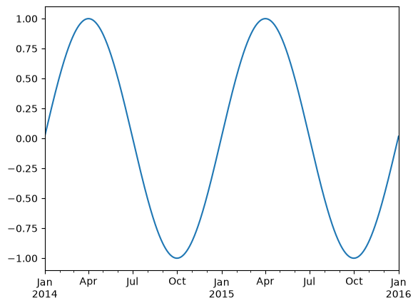
To build a time-indexed Series we first need a sequence of dates. pd.date_range generates one for us: we give it a start and end date and a frequency freq (here 'D' for one timestamp per day), and it returns a DatetimeIndex of evenly spaced timestamps. Below we make two years of daily dates, then use them as the index of a Series whose values trace a seasonal sine wave — .dayofyear counts 1–365 through the year, so one full cycle spans a year:

two_years = pd.date_range(start='2014-01-01', end='2016-01-01', freq='D')
timeseries = pd.Series(np.sin(2 *np.pi *two_years.dayofyear / 365),
                       index=two_years)
timeseries.plot()

<Axes: >

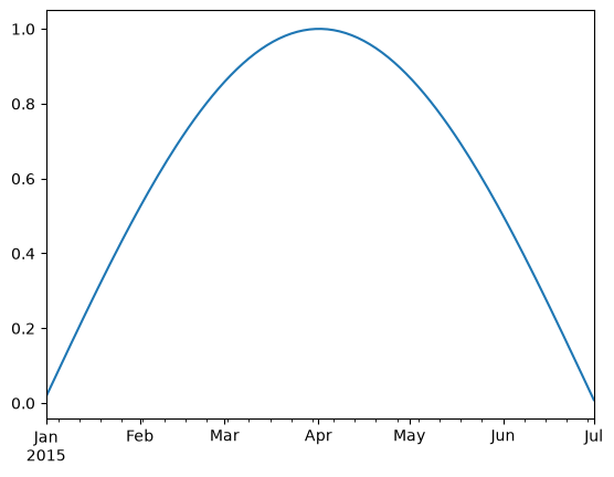
We can use python’s slicing notation inside .loc to select a date range.

timeseries.loc['2015-01-01':'2015-07-01'].plot()

<Axes: >

The TimeIndex object has lots of useful attributes

timeseries.index.month

Index([ 1,  1,  1,  1,  1,  1,  1,  1,  1,  1,
       ...
       12, 12, 12, 12, 12, 12, 12, 12, 12,  1],
      dtype='int32', length=731)

timeseries.index.day

Index([ 1,  2,  3,  4,  5,  6,  7,  8,  9, 10,
       ...
       23, 24, 25, 26, 27, 28, 29, 30, 31,  1],
      dtype='int32', length=731)

Try it

Use pd.date_range(start='2023-01-01', end='2023-12-31', freq='D') to create a year of daily timestamps. Wrap them in a Series whose values are np.random.randn(len(...)). Slice it to get just March through May 2023 (use .loc['2023-03':'2023-05']), then call .plot().

Reading Data Files: Weather Station Data

In this example, we will use NOAA weather station data from https://www.ncdc.noaa.gov/data-access/land-based-station-data.

The details of files we are going to read are described in this README file (ftp://ftp.ncdc.noaa.gov/pub/data/uscrn/products/daily01/README.txt).

import pooch
POOCH = pooch.create(
    path=pooch.os_cache("noaa-data"),
    base_url="doi:10.5281/zenodo.5564850/",
    registry={
        "data.txt": "md5:5129dcfd19300eb8d4d8d1673fcfbcb4",
    },
)
datafile = POOCH.fetch("data.txt")
datafile

Downloading file 'data.txt' from 'doi:10.5281/zenodo.5564850/data.txt' to '/home/runner/.cache/noaa-data'.

'/home/runner/.cache/noaa-data/data.txt'

! head {datafile}

WBANNO LST_DATE CRX_VN LONGITUDE LATITUDE T_DAILY_MAX T_DAILY_MIN T_DAILY_MEAN T_DAILY_AVG P_DAILY_CALC SOLARAD_DAILY SUR_TEMP_DAILY_TYPE SUR_TEMP_DAILY_MAX SUR_TEMP_DAILY_MIN SUR_TEMP_DAILY_AVG RH_DAILY_MAX RH_DAILY_MIN RH_DAILY_AVG SOIL_MOISTURE_5_DAILY SOIL_MOISTURE_10_DAILY SOIL_MOISTURE_20_DAILY SOIL_MOISTURE_50_DAILY SOIL_MOISTURE_100_DAILY SOIL_TEMP_5_DAILY SOIL_TEMP_10_DAILY SOIL_TEMP_20_DAILY SOIL_TEMP_50_DAILY SOIL_TEMP_100_DAILY 
64756 20170101  2.422  -73.74   41.79     6.6    -5.4     0.6     2.2     0.0     8.68 C     7.9    -6.6    -0.5    84.8    30.7    53.7 -99.000 -99.000   0.207   0.152   0.175    -0.1     0.0     0.6     1.5     3.4
64756 20170102  2.422  -73.74   41.79     4.0    -6.8    -1.4    -1.2     0.0     2.08 C     4.1    -7.1    -1.6    91.1    49.1    77.4 -99.000 -99.000   0.205   0.151   0.173    -0.2     0.0     0.6     1.5     3.3
64756 20170103  2.422  -73.74   41.79     4.9     0.7     2.8     2.7    13.1     0.68 C     3.9     0.1     1.6    96.5    80.1    91.5 -99.000 -99.000   0.205   0.150   0.173    -0.1     0.0     0.5     1.5     3.3
64756 20170104  2.422  -73.74   41.79     8.7    -1.6     3.6     3.5     1.3     2.85 C     9.4    -4.5     1.3    97.4    34.0    73.1 -99.000 -99.000   0.215   0.153   0.174    -0.1     0.0     0.5     1.5     3.2
64756 20170105  2.422  -73.74   41.79    -0.5    -4.6    -2.5    -2.8     0.0     4.90 C     5.0    -7.6    -3.3    51.0    34.4    42.5 -99.000 -99.000   0.215   0.154   0.177    -0.1     0.0     0.5     1.4     3.1
64756 20170106  2.422  -73.74   41.79    -2.5   -10.1    -6.3    -4.7     1.3     5.17 C     1.8   -12.9    -5.2    89.8    40.0    60.8 -99.000 -99.000   0.210   0.153   0.177    -0.2     0.0     0.5     1.4     3.1
64756 20170107  2.422  -73.74   41.79    -7.3   -11.7    -9.5    -8.7     3.1     1.19 C    -5.0   -19.0    -8.5    84.4    50.9    71.2 -99.000 -99.000   0.204   0.152   0.175    -0.4    -0.1     0.5     1.4     3.0
64756 20170108  2.422  -73.74   41.79    -5.9   -14.5   -10.2    -9.4     0.0     6.15 C    -5.5   -23.1   -14.0    76.9    40.3    59.8 -99.000 -99.000   0.206   0.150   0.175    -0.4    -0.2     0.4     1.4     3.0
64756 20170109  2.422  -73.74   41.79    -6.5   -20.2   -13.3   -12.5     0.0     5.86 C    -6.4   -23.4   -16.2    82.5    45.1    65.8 -99.000 -99.000   0.223   0.148   0.175    -0.7    -0.4     0.4     1.3     3.0

We now have a text file on our hard drive called data.txt. Examine it.

To read it into pandas, we will use the read_csv function. This function is incredibly complex and powerful. You can use it to extract data from almost any text file. However, you need to understand how to use its various options.

With no options, this is what we get.

df = pd.read_csv(datafile)
df.head()

	WBANNO LST_DATE CRX_VN LONGITUDE LATITUDE T_DAILY_MAX T_DAILY_MIN T_DAILY_MEAN T_DAILY_AVG P_DAILY_CALC SOLARAD_DAILY SUR_TEMP_DAILY_TYPE SUR_TEMP_DAILY_MAX SUR_TEMP_DAILY_MIN SUR_TEMP_DAILY_AVG RH_DAILY_MAX RH_DAILY_MIN RH_DAILY_AVG SOIL_MOISTURE_5_DAILY SOIL_MOISTURE_10_DAILY SOIL_MOISTURE_20_DAILY SOIL_MOISTURE_50_DAILY SOIL_MOISTURE_100_DAILY SOIL_TEMP_5_DAILY SOIL_TEMP_10_DAILY SOIL_TEMP_20_DAILY SOIL_TEMP_50_DAILY SOIL_TEMP_100_DAILY
0	64756 20170101  2.422  -73.74   41.79     6.6 ...
1	64756 20170102  2.422  -73.74   41.79     4.0 ...
2	64756 20170103  2.422  -73.74   41.79     4.9 ...
3	64756 20170104  2.422  -73.74   41.79     8.7 ...
4	64756 20170105  2.422  -73.74   41.79    -0.5 ...

Pandas failed to identify the different columns. This is because it expected a standard CSV (comma-separated values) file, but in our file the values are separated by whitespace instead — and not by a single space: the amount of whitespace between columns varies. We tell pandas how the columns are separated with the sep keyword.

The value r'\s+' is a small regular expression — a pattern for matching text. Here \s stands for any whitespace character (a space or a tab) and + means “one or more in a row,” so together they match any run of whitespace, however wide. The leading r makes it a raw string, which tells Python to leave the backslash alone instead of treating it as a special character.

df = pd.read_csv(datafile, sep=r'\s+')
df.head()

	WBANNO	LST_DATE	CRX_VN	LONGITUDE	LATITUDE	T_DAILY_MAX	T_DAILY_MIN	T_DAILY_MEAN	T_DAILY_AVG	P_DAILY_CALC	...	SOIL_MOISTURE_5_DAILY	SOIL_MOISTURE_10_DAILY	SOIL_MOISTURE_20_DAILY	SOIL_MOISTURE_50_DAILY	SOIL_MOISTURE_100_DAILY	SOIL_TEMP_5_DAILY	SOIL_TEMP_10_DAILY	SOIL_TEMP_20_DAILY	SOIL_TEMP_50_DAILY	SOIL_TEMP_100_DAILY
0	64756	20170101	2.422	-73.74	41.79	6.6	-5.4	0.6	2.2	0.0	...	-99.0	-99.0	0.207	0.152	0.175	-0.1	0.0	0.6	1.5	3.4
1	64756	20170102	2.422	-73.74	41.79	4.0	-6.8	-1.4	-1.2	0.0	...	-99.0	-99.0	0.205	0.151	0.173	-0.2	0.0	0.6	1.5	3.3
2	64756	20170103	2.422	-73.74	41.79	4.9	0.7	2.8	2.7	13.1	...	-99.0	-99.0	0.205	0.150	0.173	-0.1	0.0	0.5	1.5	3.3
3	64756	20170104	2.422	-73.74	41.79	8.7	-1.6	3.6	3.5	1.3	...	-99.0	-99.0	0.215	0.153	0.174	-0.1	0.0	0.5	1.5	3.2
4	64756	20170105	2.422	-73.74	41.79	-0.5	-4.6	-2.5	-2.8	0.0	...	-99.0	-99.0	0.215	0.154	0.177	-0.1	0.0	0.5	1.4	3.1

5 rows × 28 columns

Great! It worked.

If we look closely, we will see there are lots of -99 and -9999 values in the file. The README file (ftp://ftp.ncdc.noaa.gov/pub/data/uscrn/products/daily01/README.txt) tells us that these are values used to represent missing data. Let’s tell this to pandas.

df = pd.read_csv(datafile, sep=r'\s+', na_values=[-9999.0, -99.0])
df.head()

	WBANNO	LST_DATE	CRX_VN	LONGITUDE	LATITUDE	T_DAILY_MAX	T_DAILY_MIN	T_DAILY_MEAN	T_DAILY_AVG	P_DAILY_CALC	...	SOIL_MOISTURE_5_DAILY	SOIL_MOISTURE_10_DAILY	SOIL_MOISTURE_20_DAILY	SOIL_MOISTURE_50_DAILY	SOIL_MOISTURE_100_DAILY	SOIL_TEMP_5_DAILY	SOIL_TEMP_10_DAILY	SOIL_TEMP_20_DAILY	SOIL_TEMP_50_DAILY	SOIL_TEMP_100_DAILY
0	64756	20170101	2.422	-73.74	41.79	6.6	-5.4	0.6	2.2	0.0	...	NaN	NaN	0.207	0.152	0.175	-0.1	0.0	0.6	1.5	3.4
1	64756	20170102	2.422	-73.74	41.79	4.0	-6.8	-1.4	-1.2	0.0	...	NaN	NaN	0.205	0.151	0.173	-0.2	0.0	0.6	1.5	3.3
2	64756	20170103	2.422	-73.74	41.79	4.9	0.7	2.8	2.7	13.1	...	NaN	NaN	0.205	0.150	0.173	-0.1	0.0	0.5	1.5	3.3
3	64756	20170104	2.422	-73.74	41.79	8.7	-1.6	3.6	3.5	1.3	...	NaN	NaN	0.215	0.153	0.174	-0.1	0.0	0.5	1.5	3.2
4	64756	20170105	2.422	-73.74	41.79	-0.5	-4.6	-2.5	-2.8	0.0	...	NaN	NaN	0.215	0.154	0.177	-0.1	0.0	0.5	1.4	3.1

5 rows × 28 columns

Great. The missing data is now represented by NaN.

What data types did pandas infer?

df.info()

<class 'pandas.DataFrame'>
RangeIndex: 365 entries, 0 to 364
Data columns (total 28 columns):
 #   Column                   Non-Null Count  Dtype  
---  ------                   --------------  -----  
 0   WBANNO                   365 non-null    int64  
 1   LST_DATE                 365 non-null    int64  
 2   CRX_VN                   365 non-null    float64
 3   LONGITUDE                365 non-null    float64
 4   LATITUDE                 365 non-null    float64
 5   T_DAILY_MAX              364 non-null    float64
 6   T_DAILY_MIN              364 non-null    float64
 7   T_DAILY_MEAN             364 non-null    float64
 8   T_DAILY_AVG              364 non-null    float64
 9   P_DAILY_CALC             364 non-null    float64
 10  SOLARAD_DAILY            364 non-null    float64
 11  SUR_TEMP_DAILY_TYPE      365 non-null    str    
 12  SUR_TEMP_DAILY_MAX       364 non-null    float64
 13  SUR_TEMP_DAILY_MIN       364 non-null    float64
 14  SUR_TEMP_DAILY_AVG       364 non-null    float64
 15  RH_DAILY_MAX             364 non-null    float64
 16  RH_DAILY_MIN             364 non-null    float64
 17  RH_DAILY_AVG             364 non-null    float64
 18  SOIL_MOISTURE_5_DAILY    317 non-null    float64
 19  SOIL_MOISTURE_10_DAILY   317 non-null    float64
 20  SOIL_MOISTURE_20_DAILY   336 non-null    float64
 21  SOIL_MOISTURE_50_DAILY   364 non-null    float64
 22  SOIL_MOISTURE_100_DAILY  359 non-null    float64
 23  SOIL_TEMP_5_DAILY        364 non-null    float64
 24  SOIL_TEMP_10_DAILY       364 non-null    float64
 25  SOIL_TEMP_20_DAILY       364 non-null    float64
 26  SOIL_TEMP_50_DAILY       364 non-null    float64
 27  SOIL_TEMP_100_DAILY      364 non-null    float64
dtypes: float64(25), int64(2), str(1)
memory usage: 80.0 KB

One problem here is that pandas did not recognize the LST_DATE column as a date. Let’s help it.

df = pd.read_csv(datafile, sep=r'\s+',
                 na_values=[-9999.0, -99.0],
                 parse_dates=[1])
df.info()

<class 'pandas.DataFrame'>
RangeIndex: 365 entries, 0 to 364
Data columns (total 28 columns):
 #   Column                   Non-Null Count  Dtype         
---  ------                   --------------  -----         
 0   WBANNO                   365 non-null    int64         
 1   LST_DATE                 365 non-null    datetime64[us]
 2   CRX_VN                   365 non-null    float64       
 3   LONGITUDE                365 non-null    float64       
 4   LATITUDE                 365 non-null    float64       
 5   T_DAILY_MAX              364 non-null    float64       
 6   T_DAILY_MIN              364 non-null    float64       
 7   T_DAILY_MEAN             364 non-null    float64       
 8   T_DAILY_AVG              364 non-null    float64       
 9   P_DAILY_CALC             364 non-null    float64       
 10  SOLARAD_DAILY            364 non-null    float64       
 11  SUR_TEMP_DAILY_TYPE      365 non-null    str           
 12  SUR_TEMP_DAILY_MAX       364 non-null    float64       
 13  SUR_TEMP_DAILY_MIN       364 non-null    float64       
 14  SUR_TEMP_DAILY_AVG       364 non-null    float64       
 15  RH_DAILY_MAX             364 non-null    float64       
 16  RH_DAILY_MIN             364 non-null    float64       
 17  RH_DAILY_AVG             364 non-null    float64       
 18  SOIL_MOISTURE_5_DAILY    317 non-null    float64       
 19  SOIL_MOISTURE_10_DAILY   317 non-null    float64       
 20  SOIL_MOISTURE_20_DAILY   336 non-null    float64       
 21  SOIL_MOISTURE_50_DAILY   364 non-null    float64       
 22  SOIL_MOISTURE_100_DAILY  359 non-null    float64       
 23  SOIL_TEMP_5_DAILY        364 non-null    float64       
 24  SOIL_TEMP_10_DAILY       364 non-null    float64       
 25  SOIL_TEMP_20_DAILY       364 non-null    float64       
 26  SOIL_TEMP_50_DAILY       364 non-null    float64       
 27  SOIL_TEMP_100_DAILY      364 non-null    float64       
dtypes: datetime64[us](1), float64(25), int64(1), str(1)
memory usage: 80.0 KB

It worked! Finally, let’s tell pandas to use the date column as the index.

df = df.set_index('LST_DATE')
df.head()

	WBANNO	CRX_VN	LONGITUDE	LATITUDE	T_DAILY_MAX	T_DAILY_MIN	T_DAILY_MEAN	T_DAILY_AVG	P_DAILY_CALC	SOLARAD_DAILY	...	SOIL_MOISTURE_5_DAILY	SOIL_MOISTURE_10_DAILY	SOIL_MOISTURE_20_DAILY	SOIL_MOISTURE_50_DAILY	SOIL_MOISTURE_100_DAILY	SOIL_TEMP_5_DAILY	SOIL_TEMP_10_DAILY	SOIL_TEMP_20_DAILY	SOIL_TEMP_50_DAILY	SOIL_TEMP_100_DAILY
LST_DATE
2017-01-01	64756	2.422	-73.74	41.79	6.6	-5.4	0.6	2.2	0.0	8.68	...	NaN	NaN	0.207	0.152	0.175	-0.1	0.0	0.6	1.5	3.4
2017-01-02	64756	2.422	-73.74	41.79	4.0	-6.8	-1.4	-1.2	0.0	2.08	...	NaN	NaN	0.205	0.151	0.173	-0.2	0.0	0.6	1.5	3.3
2017-01-03	64756	2.422	-73.74	41.79	4.9	0.7	2.8	2.7	13.1	0.68	...	NaN	NaN	0.205	0.150	0.173	-0.1	0.0	0.5	1.5	3.3
2017-01-04	64756	2.422	-73.74	41.79	8.7	-1.6	3.6	3.5	1.3	2.85	...	NaN	NaN	0.215	0.153	0.174	-0.1	0.0	0.5	1.5	3.2
2017-01-05	64756	2.422	-73.74	41.79	-0.5	-4.6	-2.5	-2.8	0.0	4.90	...	NaN	NaN	0.215	0.154	0.177	-0.1	0.0	0.5	1.4	3.1

5 rows × 27 columns

We can now access values by time:

df.loc['2017-08-07']

WBANNO                     64756
CRX_VN                     2.422
LONGITUDE                 -73.74
LATITUDE                   41.79
T_DAILY_MAX                 19.3
T_DAILY_MIN                 12.3
T_DAILY_MEAN                15.8
T_DAILY_AVG                 16.3
P_DAILY_CALC                 4.9
SOLARAD_DAILY               3.93
SUR_TEMP_DAILY_TYPE            C
SUR_TEMP_DAILY_MAX          22.3
SUR_TEMP_DAILY_MIN          11.9
SUR_TEMP_DAILY_AVG          17.7
RH_DAILY_MAX                94.7
RH_DAILY_MIN                76.4
RH_DAILY_AVG                89.5
SOIL_MOISTURE_5_DAILY      0.148
SOIL_MOISTURE_10_DAILY     0.113
SOIL_MOISTURE_20_DAILY     0.094
SOIL_MOISTURE_50_DAILY     0.114
SOIL_MOISTURE_100_DAILY    0.151
SOIL_TEMP_5_DAILY           21.4
SOIL_TEMP_10_DAILY          21.7
SOIL_TEMP_20_DAILY          22.1
SOIL_TEMP_50_DAILY          22.2
SOIL_TEMP_100_DAILY         21.5
Name: 2017-08-07 00:00:00, dtype: object

Or use slicing to get a range:

df.loc['2017-07-01':'2017-07-31']

	WBANNO	CRX_VN	LONGITUDE	LATITUDE	T_DAILY_MAX	T_DAILY_MIN	T_DAILY_MEAN	T_DAILY_AVG	P_DAILY_CALC	SOLARAD_DAILY	...	SOIL_MOISTURE_5_DAILY	SOIL_MOISTURE_10_DAILY	SOIL_MOISTURE_20_DAILY	SOIL_MOISTURE_50_DAILY	SOIL_MOISTURE_100_DAILY	SOIL_TEMP_5_DAILY	SOIL_TEMP_10_DAILY	SOIL_TEMP_20_DAILY	SOIL_TEMP_50_DAILY	SOIL_TEMP_100_DAILY
LST_DATE
2017-07-01	64756	2.422	-73.74	41.79	28.0	19.7	23.9	23.8	0.2	19.28	...	0.157	0.136	0.144	0.129	0.163	25.7	25.4	23.7	21.9	19.9
2017-07-02	64756	2.422	-73.74	41.79	29.8	18.4	24.1	23.7	4.0	27.67	...	0.146	0.135	0.143	0.129	0.162	26.8	26.4	24.5	22.3	20.1
2017-07-03	64756	2.422	-73.74	41.79	28.3	15.0	21.7	21.4	0.0	27.08	...	0.141	0.132	0.139	0.128	0.162	26.4	26.3	24.8	22.8	20.3
2017-07-04	64756	2.422	-73.74	41.79	26.8	12.6	19.7	20.0	0.0	29.45	...	0.131	0.126	0.136	0.126	0.161	25.9	25.8	24.6	22.9	20.6
2017-07-05	64756	2.422	-73.74	41.79	28.0	11.9	20.0	20.7	0.0	26.90	...	0.116	0.114	0.131	0.125	0.161	25.3	25.3	24.2	22.8	20.7
2017-07-06	64756	2.422	-73.74	41.79	25.7	14.3	20.0	20.3	0.0	19.03	...	0.105	0.104	0.126	0.124	0.160	24.7	24.7	23.9	22.7	20.9
2017-07-07	64756	2.422	-73.74	41.79	25.8	16.8	21.3	20.0	11.5	13.88	...	0.114	0.100	0.123	0.123	0.160	24.2	24.2	23.4	22.4	20.8
2017-07-08	64756	2.422	-73.74	41.79	29.0	15.3	22.1	21.5	0.0	21.92	...	0.130	0.106	0.122	0.123	0.159	25.5	25.3	23.9	22.4	20.8
2017-07-09	64756	2.422	-73.74	41.79	26.3	10.9	18.6	19.4	0.0	29.72	...	0.119	0.103	0.119	0.121	0.158	24.8	24.8	23.8	22.5	20.8
2017-07-10	64756	2.422	-73.74	41.79	27.6	11.8	19.7	21.3	0.0	23.67	...	0.105	0.096	0.113	0.120	0.158	24.7	24.7	23.6	22.5	20.9
2017-07-11	64756	2.422	-73.74	41.79	27.4	19.2	23.3	22.6	8.5	17.79	...	0.106	0.093	0.110	0.120	0.157	25.6	25.4	24.1	22.6	20.9
2017-07-12	64756	2.422	-73.74	41.79	29.4	18.5	23.9	23.1	1.9	16.27	...	0.108	0.094	0.108	0.118	0.157	25.8	25.6	24.2	22.8	21.0
2017-07-13	64756	2.422	-73.74	41.79	29.5	18.3	23.9	23.4	23.3	13.61	...	0.134	0.110	0.108	0.118	0.156	25.7	25.7	24.4	23.0	21.0
2017-07-14	64756	2.422	-73.74	41.79	18.5	15.9	17.2	17.5	4.1	5.36	...	0.194	0.151	0.114	0.120	0.155	23.0	23.3	23.4	22.9	21.2
2017-07-15	64756	2.422	-73.74	41.79	26.6	16.5	21.5	21.0	0.8	21.13	...	0.190	0.163	0.119	0.122	0.155	24.6	24.4	23.2	22.2	21.2
2017-07-16	64756	2.422	-73.74	41.79	27.9	13.3	20.6	21.0	0.0	27.03	...	0.171	0.154	0.123	0.123	0.155	25.4	25.3	23.9	22.6	21.1
2017-07-17	64756	2.422	-73.74	41.79	29.2	16.1	22.6	22.9	0.0	20.47	...	0.155	0.143	0.124	0.122	0.156	25.7	25.6	24.4	22.9	21.2
2017-07-18	64756	2.422	-73.74	41.79	30.3	19.3	24.8	24.7	0.0	24.99	...	0.142	0.132	0.122	0.122	0.156	27.0	26.7	24.9	23.2	21.3
2017-07-19	64756	2.422	-73.74	41.79	31.2	19.1	25.1	25.0	0.0	27.69	...	0.126	0.118	0.118	0.122	0.156	27.6	27.4	25.6	23.7	21.5
2017-07-20	64756	2.422	-73.74	41.79	31.8	16.6	24.2	23.4	0.7	21.53	...	0.111	0.103	0.114	0.121	0.156	27.0	27.0	25.6	24.0	21.7
2017-07-21	64756	2.422	-73.74	41.79	30.6	16.6	23.6	23.6	0.0	25.55	...	0.100	0.093	0.108	0.120	0.155	27.1	27.0	25.5	24.0	21.9
2017-07-22	64756	2.422	-73.74	41.79	27.7	15.6	21.7	21.2	0.5	16.04	...	0.092	0.086	0.104	0.119	0.156	25.9	26.1	25.3	24.1	22.0
2017-07-23	64756	2.422	-73.74	41.79	26.4	18.5	22.5	22.2	0.0	19.03	...	0.087	0.082	0.100	0.118	0.155	26.0	26.0	24.9	23.8	22.1
2017-07-24	64756	2.422	-73.74	41.79	19.4	14.8	17.1	16.7	29.2	9.10	...	0.145	0.118	0.102	0.117	0.154	23.1	23.6	23.9	23.5	22.1
2017-07-25	64756	2.422	-73.74	41.79	18.6	13.7	16.2	16.2	0.0	7.35	...	0.167	0.133	0.107	0.116	0.153	21.9	22.2	22.4	22.5	21.9
2017-07-26	64756	2.422	-73.74	41.79	24.7	11.2	18.0	18.3	0.0	22.22	...	0.155	0.128	0.108	0.118	0.152	22.9	23.0	22.3	22.0	21.7
2017-07-27	64756	2.422	-73.74	41.79	24.2	15.2	19.7	19.5	0.0	8.28	...	0.144	0.122	0.109	0.118	0.154	22.5	22.7	22.4	22.0	21.4
2017-07-28	64756	2.422	-73.74	41.79	26.5	16.9	21.7	20.9	0.0	21.06	...	0.137	0.117	0.110	0.119	0.154	24.1	24.1	22.8	22.0	21.3
2017-07-29	64756	2.422	-73.74	41.79	24.2	10.4	17.3	18.1	0.0	21.28	...	0.126	0.108	0.108	0.118	0.154	23.3	23.6	23.0	22.2	21.3
2017-07-30	64756	2.422	-73.74	41.79	25.5	8.2	16.8	17.3	0.0	27.68	...	0.113	0.099	0.104	0.117	0.154	22.8	23.0	22.4	22.0	21.3
2017-07-31	64756	2.422	-73.74	41.79	29.4	10.1	19.7	20.1	0.0	25.49	...	0.101	0.090	0.099	0.116	0.153	23.8	23.8	22.7	21.9	21.2

31 rows × 27 columns

Quick Statistics

describe() is a fast way to get a feel for a freshly loaded dataset: in one call it reports the count, mean, standard deviation, minimum, the 25/50/75% percentiles, and maximum for every numeric column. It’s a good first sanity check — unrealistic values or columns full of NaN often jump out right away.

df.describe()

	WBANNO	CRX_VN	LONGITUDE	LATITUDE	T_DAILY_MAX	T_DAILY_MIN	T_DAILY_MEAN	T_DAILY_AVG	P_DAILY_CALC	SOLARAD_DAILY	...	SOIL_MOISTURE_5_DAILY	SOIL_MOISTURE_10_DAILY	SOIL_MOISTURE_20_DAILY	SOIL_MOISTURE_50_DAILY	SOIL_MOISTURE_100_DAILY	SOIL_TEMP_5_DAILY	SOIL_TEMP_10_DAILY	SOIL_TEMP_20_DAILY	SOIL_TEMP_50_DAILY	SOIL_TEMP_100_DAILY
count	365.0	365.000000	365.00	3.650000e+02	364.000000	364.000000	364.000000	364.000000	364.000000	364.000000	...	317.000000	317.000000	336.000000	364.000000	359.000000	364.000000	364.000000	364.000000	364.000000	364.000000
mean	64756.0	2.470767	-73.74	4.179000e+01	15.720055	4.037912	9.876374	9.990110	2.797802	13.068187	...	0.189498	0.183991	0.165470	0.140192	0.160630	12.312637	12.320604	12.060165	11.978022	11.915659
std	0.0	0.085997	0.00	7.115181e-15	10.502087	9.460676	9.727451	9.619168	7.238628	7.953074	...	0.052031	0.054113	0.043989	0.020495	0.016011	9.390034	9.338176	8.767752	8.078346	7.187317
min	64756.0	2.422000	-73.74	4.179000e+01	-12.300000	-21.800000	-17.000000	-16.700000	0.000000	0.100000	...	0.075000	0.078000	0.087000	0.101000	0.117000	-0.700000	-0.400000	0.200000	0.900000	1.900000
25%	64756.0	2.422000	-73.74	4.179000e+01	6.900000	-2.775000	2.100000	2.275000	0.000000	6.225000	...	0.152000	0.139000	0.118750	0.118000	0.154000	2.225000	2.000000	2.475000	3.300000	4.100000
50%	64756.0	2.422000	-73.74	4.179000e+01	17.450000	4.350000	10.850000	11.050000	0.000000	12.865000	...	0.192000	0.198000	0.183000	0.147500	0.165000	13.300000	13.350000	13.100000	12.850000	11.600000
75%	64756.0	2.422000	-73.74	4.179000e+01	24.850000	11.900000	18.150000	18.450000	1.400000	19.740000	...	0.234000	0.227000	0.203000	0.157000	0.173000	21.025000	21.125000	20.400000	19.800000	19.325000
max	64756.0	2.622000	-73.74	4.179000e+01	33.400000	20.700000	25.700000	26.700000	65.700000	29.910000	...	0.296000	0.321000	0.235000	0.182000	0.192000	27.600000	27.400000	25.600000	24.100000	22.100000

8 rows × 26 columns

Plotting Values

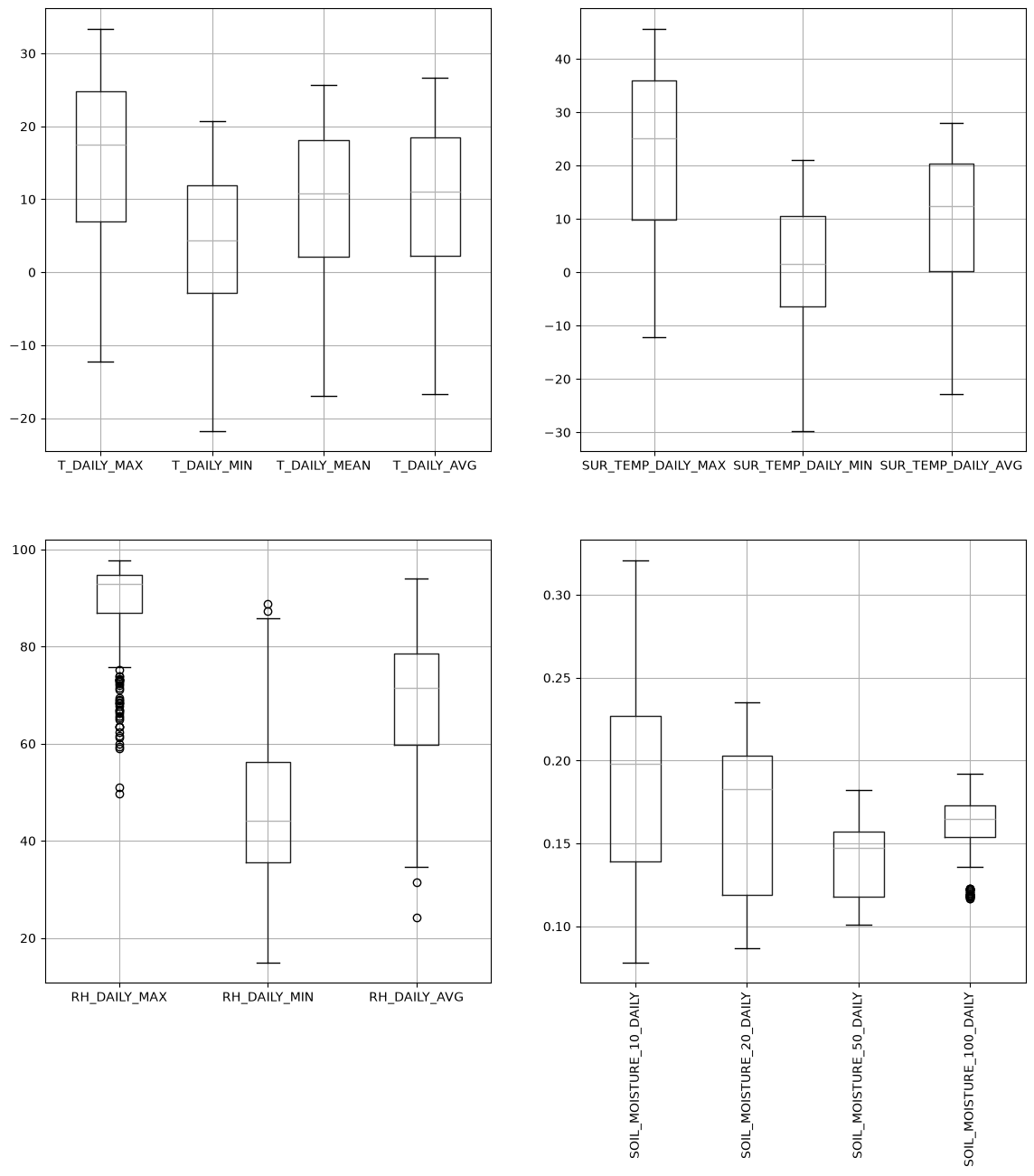
We can now quickly make plots of the data

fig, ax = plt.subplots(ncols=2, nrows=2, figsize=(14,14))

df.iloc[:, 4:8].boxplot(ax=ax[0,0])
df.iloc[:, 10:14].boxplot(ax=ax[0,1])
df.iloc[:, 14:17].boxplot(ax=ax[1,0])
df.iloc[:, 18:22].boxplot(ax=ax[1,1])


ax[1, 1].set_xticklabels(ax[1, 1].get_xticklabels(), rotation=90);

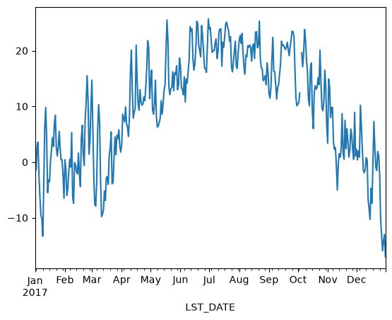
Pandas is very “time aware”:

df.T_DAILY_MEAN.plot()

<Axes: xlabel='LST_DATE'>

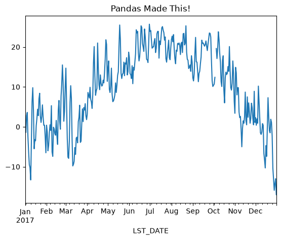
Note: we could also manually create an axis and plot into it.

fig, ax = plt.subplots()
df.T_DAILY_MEAN.plot(ax=ax)
ax.set_title('Pandas Made This!')

Text(0.5, 1.0, 'Pandas Made This!')

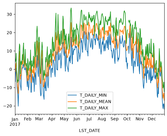
df[['T_DAILY_MIN', 'T_DAILY_MEAN', 'T_DAILY_MAX']].plot()

<Axes: xlabel='LST_DATE'>

Try it

Slice the NOAA df to a single month of your choice (e.g., df.loc['2018-06']). Call .describe() on that subset to get summary stats. Then plot T_DAILY_MEAN against the index for that month.

Resampling

Because pandas understands time, it can resample a time series — change how often the data is reported by grouping together all the timestamps that fall in each new time period. Our data is daily, but we might want monthly values; resampling to a monthly frequency gathers all the days in each month so we can summarize them (mean, max, …). It’s much like groupby, except the groups are consecutive time intervals. The target frequency is given by a short code — below, 'MS' means “month start” (one value per month); other common codes are 'D' (daily), 'W' (weekly), and 'YE' (year end).

Calling .resample(...) returns a resampler object — a grouping by time frequency. Apply an aggregation (like .mean()) to actually get a smaller DataFrame:

rs_obj = df.select_dtypes(include='number').resample('MS')
rs_obj

<pandas.core.resample.DatetimeIndexResampler object at 0x7f7ca561b4d0>

rs_obj.mean()

	WBANNO	CRX_VN	LONGITUDE	LATITUDE	T_DAILY_MAX	T_DAILY_MIN	T_DAILY_MEAN	T_DAILY_AVG	P_DAILY_CALC	SOLARAD_DAILY	...	SOIL_MOISTURE_5_DAILY	SOIL_MOISTURE_10_DAILY	SOIL_MOISTURE_20_DAILY	SOIL_MOISTURE_50_DAILY	SOIL_MOISTURE_100_DAILY	SOIL_TEMP_5_DAILY	SOIL_TEMP_10_DAILY	SOIL_TEMP_20_DAILY	SOIL_TEMP_50_DAILY	SOIL_TEMP_100_DAILY
LST_DATE
2017-01-01	64756.0	2.422000	-73.74	41.79	3.945161	-3.993548	-0.025806	0.038710	3.090323	4.690000	...	0.236900	0.248300	0.204550	0.152806	0.175194	0.209677	0.267742	0.696774	1.438710	2.877419
2017-02-01	64756.0	2.422000	-73.74	41.79	7.246429	-4.360714	1.442857	1.839286	2.414286	10.364286	...	0.226333	0.243000	0.207545	0.152857	0.175786	1.125000	1.100000	1.192857	1.492857	2.367857
2017-03-01	64756.0	2.422000	-73.74	41.79	5.164516	-5.335484	-0.090323	0.167742	3.970968	13.113548	...	0.218033	0.229267	0.196258	0.153484	0.174548	2.122581	2.161290	2.345161	2.700000	3.387097
2017-04-01	64756.0	2.422000	-73.74	41.79	17.813333	5.170000	11.493333	11.540000	2.300000	14.645000	...	0.199733	0.210300	0.190667	0.151000	0.172400	11.066667	10.666667	9.636667	8.426667	6.903333
2017-05-01	64756.0	2.422000	-73.74	41.79	19.151613	7.338710	13.229032	13.638710	4.141935	16.519677	...	0.206613	0.210935	0.185613	0.147710	0.170000	16.454839	16.290323	15.361290	14.270968	12.696774
2017-06-01	64756.0	2.422000	-73.74	41.79	25.423333	12.176667	18.796667	18.986667	3.743333	21.655000	...	0.185167	0.184300	0.173167	0.142533	0.167000	22.350000	22.166667	20.880000	19.370000	17.333333
2017-07-01	64756.0	2.422000	-73.74	41.79	26.912903	15.183871	21.048387	20.993548	2.732258	20.566129	...	0.131226	0.115774	0.116613	0.121032	0.156677	24.993548	24.980645	23.925806	22.745161	21.164516
2017-08-01	64756.0	2.422000	-73.74	41.79	25.741935	12.954839	19.351613	19.477419	2.758065	18.360000	...	0.143871	0.122258	0.105452	0.115290	0.151034	23.374194	23.519355	22.848387	22.193548	21.377419
2017-09-01	64756.0	2.422000	-73.74	41.79	24.186667	11.300000	17.746667	17.463333	1.893333	15.154667	...	0.145167	0.139633	0.117267	0.112167	0.141926	20.256667	20.386667	19.966667	19.766667	19.530000
2017-10-01	64756.0	2.602645	-73.74	41.79	21.043333	7.150000	14.100000	13.976667	3.500000	10.395000	...	0.151767	0.137767	0.111900	0.108900	0.122067	16.086667	16.193333	16.370000	16.893333	17.386667
2017-11-01	64756.0	2.622000	-73.74	41.79	10.346667	-2.093333	4.120000	4.336667	0.826667	6.723333	...	0.241633	0.224467	0.203367	0.159500	0.155233	7.056667	7.273333	8.043333	9.633333	11.440000
2017-12-01	64756.0	2.622000	-73.74	41.79	1.496774	-7.412903	-2.967742	-2.838710	2.109677	4.474194	...	0.255929	0.239071	0.213258	0.165387	0.163290	2.064516	2.241935	2.874194	4.248387	6.019355

12 rows × 26 columns

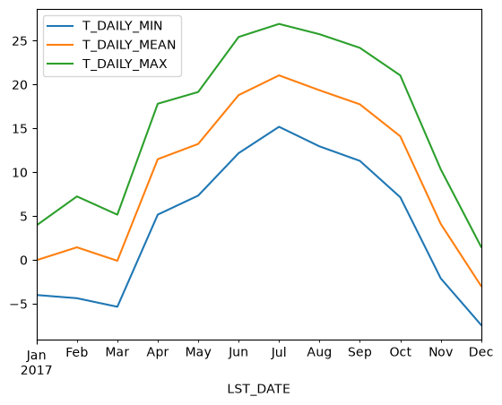
We can chain all of that together

df_mm = df.select_dtypes(include='number').resample('MS').mean()
df_mm[['T_DAILY_MIN', 'T_DAILY_MEAN', 'T_DAILY_MAX']].plot()

<Axes: xlabel='LST_DATE'>

Try it

Use df.resample('YE').mean() to get yearly means and plot T_DAILY_MAX against the resulting index as a line chart. Then do the same with '10D' (10-day bins) — the lower-frequency series should look smoother.

Recap

You’ve now met the two core pandas objects and the everyday ways to work with them:

• Series and DataFrames — labelled 1-D and 2-D data, with .info() and .describe() for a quick look.

• Indexing — .loc (by label), .iloc (by position), and boolean masks to filter rows by a condition.

• Building and combining — adding computed columns, and joining a Series or DataFrame on a shared index.

• Reading real data — read_csv with sep, na_values, and parse_dates, then setting a column as the index.

• Time series — a DatetimeIndex, slicing by date, plotting straight from a DataFrame, and a first taste of resample.

Next we go deeper into grouping operations — groupby, resample, and rolling — in Pandas: Groupby.